info

intro

Java 11
日志框架 the Apache Log4j 2 framework
测试框架 the TestNG framework
测试覆盖率 the JaCoCo library
测试调试 -DforkMode=never
SQL 解析 the ANTLR parsing framework

lab1

基本流程

// 初始化数据库
ExclusiveClient.startup
NanoDBServer.startup
StorageManager.initialize

// 解析命令
InteractiveClient.mainloop
InteractiveClient.processEnteredText
ExclusiveClient.handleCommand
NanoDBServer.doCommand(String, boolean)
NanoDBServer.parseCommand
NanoDBServer.doCommand(Command, boolean)

create table 流程

// 执行命令
CreateTableCommand.execute
CreateTableCommand.initTableConstraints
IndexedTableManager.createTable
FileManagerImpl.createDBFile
HeapTupleFileManager.createTupleFile
HeapTupleFileManager.saveMetadata
SchemaWriter.writeSchema
StatsWriter.writeTableStats

insert 流程

// 执行命令
InsertCommand.execute
InsertCommand.insertSingleRow
HeapTupleFile.addTuple
DataPage.allocNewTuple
HeapFilePageTuple.storeNewTuple
PageTuple.storeTuple

update 流程

// 执行命令
QueryCommand.execute
QueryEvaluator.executePlan
TupleUpdater.process
HeapTupleFile.updateTuple
HeapFilePageTuple.setColumnValue

delete 流程

// 执行命令
QueryCommand.execute
QueryEvaluator.executePlan
TupleRemover.process
HeapTupleFile.deleteTuple
DataPage.deleteTuple

NanoDB Tuple Updates and Deletion

删除较为简单，修改 DataPage.deleteTuple 方法

使用 deleteTupleDataRange 删除数据

[tupDataStart, off) -> [tupDataStart + len, off + len)

置对应的 slot 为 EMPTY_SLOT

最后删除 header 尾部的空 slots 即可

此时可以通过如下测试

testHeapTableMultiPageInsert
testHeapTableMultiPageInsertDelete
testHeapTableOnePageInsert
testHeapTableOnePageInsertDelete
testInsertDeleteManyTimes

更新较为繁琐，首先了解一下 tuple 的布局，data page 的布局如下

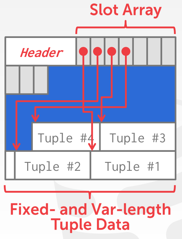
在每个 tuple 的开头处，会有一段 bitmap 指示该 tuple 的各字段是否为 null

例如，对于这样的 schema

CREATE TABLE heap_update (a INTEGER, b BIGINT, c CHAR(7), d DOUBLE, e VARCHAR(20), f FLOAT);

插入三个 tuples 后，各字段的 offset 如下

[8067, 8071, 8079, 8086, 8094, 8109] - tuple3
[8114, 8118, 8126, 8133, 8141, 8147] - tuple2
[8152, 8156, 8164, 8171, 8179, 8188] - tuple1

注意 tuple1 的 pageOffset 为 8151，这里存放了一个字节的 bitmap，所以其第一个字段的 offset 为 8152

各字段之间紧密排列，不存在 gap

tricky 的地方在于扩缩容，使用 deleteTupleDataRange 缩容，使用 insertTupleDataRange 扩容，注意扩容的变化

[tupDataStart, off) -> [tupDataStart - len, off - len)

也就是扩容后新增的空间位于 [off - len, off)

需要手动维护 pageOffset，以便于在最后调用 computeValueOffsets 更新各字段的 offsets

同时，扩缩容也会修改 slot array，不必考虑 slot 的设置是否正确

其余 tuple 的 pageOffset 可能随 slot 的设置动态变化，所以不必考虑

此时可以通过如下测试

testUpdates

NanoDB Buffer Management

主要考虑 page 和 tuple 的 pin 问题

DBPage 和 PageTuple 类均实现了 Pinnable 接口

其中对 PageTuple 的 pin 和 unpin 会影响包含该 tuple 的 DBPage

主要修改如下地方

HeapTupleFile.java

参考 getFirstTuple 方法，为 getTuple / getNextTuple / addTuple 方法添加 unpin page 调用

注意这里不必修改 updateTuple 和 deleteTuple 方法

HeapTupleFileManager.java

修改 openTupleFile 和 saveMetadata 方法，添加 unpin header page 调用

QueryEvaluator.java

在 process 前 pin tuple，在 process 后 unpin tuple

注意这里的 process 可能会调用 updateTuple 和 deleteTuple 方法，并且是唯一调用点，所以可以通过调用者来管理

SelectNode.java

其 getNextTuple 方法实现了 PlanNode 的 getNextTuple 方法

而 QueryEvaluator 在 executePlan 时会调用 getNextTuple 方法

SelectNode 的 getNextTuple 方法会调用 advanceCurrentTuple 获取新的 tuple，其实现会调用 getFirstTuple 和 getNextTuple 方法

而上文已经实现了 page 层面的 pin 和 unpin，所以感觉不必添加新的代码

实现之后，可以使用如下命令进行大规模测试

rm datafiles/*
./nanodb < schemas/insert-perf/make-insperf.sql
./nanodb < schemas/insert-perf/ins20k.sql

若未实现，会报错 Not enough room to allocate a buffer of 8192 bytes!

可以在 sql 文件的 EXIT; 前添加 SHOW 'STORAGE' STATS;，以检查存储性能

NanoDB Storage Performance

初始性能

$ ./nanodb < schemas/insert-perf/ins20k.sql
storage.pagesRead = 3306267
storage.pagesWritten = 20000
storage.fileChanges = 1
storage.fileDistanceTraveled = 105144752

StorageManager 通过 baseDir 构造 FileManager，再通过 FileManager 构造 BufferManager

FileManager 在 loadPage 和 savePage 时，会通过 updateFileIOPerfStats 更新统计数据

以 StorageManager 的 loadDBPage 为例，会调用 BufferManager 的 getPage，其中调用了 FileManager 的 loadPage

每一个 table 对应一个 DBFile，每一个 DBFile 包含多个 DBPage，第一个 page 为 HeaderPage，其余为 DataPage

以 heap tuple file 为例，HeaderPage 的布局如下

file type
page size
schema size
stats size
schema
stats

DataPage 的布局上面已经讲过了，其 header 只保存 slot number 信息

由于每次 insert tuple 时，都会从第一个 data page 开始，遍历每一个空间足够的 page 的每一个 slot

这里的所需的空间包括 tuple 的大小，并且假定需要分配新的 slot

所以时间效率较低，但空间效率极高

有一个非常简单的想法，考虑每次 insert tuple 时，都从最后一个 data page 开始，也就是 append-only

int pageNo = Math.max(1, dbFile.getNumPages() - 1);

性能如下

storage.pagesRead = 20664
storage.pagesWritten = 20000
storage.fileChanges = 1
storage.fileDistanceTraveled = 5312

在 delete 操作较多时，会带来空间的浪费

突然发现 insert_perf.tbl 的大小和 ins20k.sql 差不多

对于文件结构的优化，暂时没有什么思路

lab2

overview

SELECT * FROM test_simple_selects WHERE b < 25

SelectCommand 为 QueryCommand 的子类

其 execute 的第一步是 prepareQueryPlan
- 其中会根据 SelectClause 计算 result schema
  - 更具体的，根据 FromClause 计算 from schema
  - 检查 SELECT value 的引用是否存在，配合 from schema 构造 result schema
  - 检查 WHERE / GROUP BY / HAVING / ORDER BY 中表达式的引用是否存在
  - 目前暂不考虑处理 SELECT 中的子查询
- 获取 properties 中指定的 planner，并调用其 makePlan 方法
  - makePlan 方法会继续调用 makeSimpleSelect 方法
    - 通过 FileScanNode 构造 PlanNode，并调用其 prepare 方法
获取 TupleProcessor，这里对应为 ResultCollector
- 其余 DML 的对应为 TupleInserter / TupleUpdater / TupleRemover
- 在 execute 调用前就已经设置好了
调用 QueryEvaluator.executePlan(plan, processor)
- 调用 PlanNode 的 initialize 方法
- 通过 PlanNode 不断获取 next tuple，并使用 TupleProcessor 处理该 tuple

features

Basic SELECT statements that involve zero or more tables being joined together. (For example, “SELECT 3 + 2 AS five;” is a valid SQL query. The project plan-node is able to support situations where it has no child plan, and no expression references a column name.) Join predicates may appear in the WHERE clause, or in an ON clause.
Basic joins using the “SELECT ... FROM t1, t2, ...” syntax, as well as joins with an ON clause. You do not need to support NATURAL joins or joins with the USING clause in this planner (although this is available as an extra-credit task).
Left- and right-outer joins using the nested-loop join node (which you will work on in the next section). You do not need to support full-outer joins.
Subqueries in the FROM clause.
Grouping and aggregation, where both grouping attributes and aggregates may be expressions, and where a given SELECT expression may include multiple aggregate operations. You are encouraged to use the supplied HashedGroupAggregateNode class. You will need to provide some limited validation of these expressions; details are given in a subsequent section.
ORDER BY clauses, using the supplied edu.caltech.nanodb.plans.SortNode class.

paradigm

PlanNode plan = null;

if (FROM-clause is present)
    plan = generate_FROM_clause_plan();

if (WHERE-clause is present)
    plan = add_WHERE_clause_to(plan);

if (GROUP-BY-clause and/or HAVING-clause is present)
    plan = handle_grouping_and_aggregation(plan);

if (ORDER-BY-clause is present)
    plan = add_ORDER_BY_clause_to(plan);

// There's always a SELECT clause of some sort!
plan = add_SELECT_clause_to(plan);

note

记录了完成上述 features 的顺序

Projection

对应的测试用例 TestSelectProject

利用 ProjectNode 即可

在 SimplePlanner 类中保留 makeSimpleSelect 方法，完全重写 makePlan 方法

No `FROM` clause

对应的测试用例 TestSimpleFunctions

考虑构造 ProjectNode 时，sub plan 为 null 的情形即可

`FROM` clause subqueries

添加测试用例 TestFromSubquery，在 test_sql.props 中进行数据的定义和插入

将新增的测试用例归类为 hw2-self，注意修改 pom.xml

根据 FromClause 的类型判断是否存在子查询

递归调用 makePlan 后，利用 RenameNode 重命名为 alias name，即 AS 子句中的 table name

注意对于 FROM clause 而言

BASE_TABLE 类型可能包含 AS 子句
SELECT_SUBQUERY 类型一定包含 AS 子句
JOIN_EXPR 类型一定不包含 AS 子句

下面解释使用 RenameNode 的必要性，考虑如下一个简单的查询

SELECT tmp.a FROM test_simple_selects AS tmp

若不使用 RenameNode，则对应的查询计划为

Project[values:  [tmp.a]]
    FileScan[table:  test_simple_selects]

在 ProjectNode prepare 的过程中，会在 FileScanNode 产生的 schema 中检查 tmp.a 的存在，而显然 schema 中只包含 test_simple_selects.a，所以会报错

而 RenameNode 在 prepare 的过程中，会修改自身 schema 的 table name 为 alias，所以可以通过 ProjectNode prepare 的检查，而其 getNextTuple 方法只是简单的调用 child 的 getNextTuple 方法

`FROM` clause join

添加测试用例 TestFromJoins

目前需要实现如下四种类型的 join

SELECT * FROM t1, t2 WHERE t1.a = t2.a - cross join with where clause
SELECT * FROM t1 JOIN t2 ON t1.a = t2.a - inner join with on expr
SELECT * FROM t1 LEFT OUTER JOIN t2 ON t1.a = t2.a - left join with on expr
SELECT * FROM t1 RIGHT OUTER JOIN t2 ON t1.a = t2.a - right join with on expr

在 makePlan 方法中，只需利用 NestedLoopJoinNode 即可

需要注意 join expr 的 child 的类型不一定是 BASE_TABLE，所以这里需要递归解析 FROM clause

关键在于 NestedLoopJoinNode 内部的实现，集中为 getTuplesToJoin 方法

首先在构造时，通过调用 swap 将 right outer join 化归为 left outer join

然后是 getTuplesToJoin 方法，思路如下

若 left table 为空，则直接 done，因为不可能为 right outer join
使用 leftTupleJoined 字段标记当前的 left tuple 是否成功 join，在消耗完 right table 时，若没有成功 join，且 join 类型为 left outer join，则生成 dangling tuple，且 dangling tuple 无视 predicate 限制

`ORDER BY` clauses

添加测试用例 TestOrderBy

利用 SortNode 即可，注意 SortNode 内部的实现是预先排序好所有的 tuples，所以当 tuple 数量较多时，可能导致内存不足

Grouping and Aggregation

对应的测试用例如下

TestAggregation
TestGroupBy
TestGroupingAndAggregation
TestHaving

利用 Expression 类的 traverse 方法，收集 select value 和 having expression 中出现的 aggregate function，建立 String 到 FunctionCall 的映射，并将 expression 转换为 ColumnValue

只要 aggregates 或 groupByExprs 不为空，则利用 HashedGroupAggregateNode 构造 plan

若存在 havingExpr，则利用 PlanUtils.addPredicateToPlan 进行筛选

考虑如下的 table

a	b	c
1	1	5
1	2	6
2	3	8
2	4	12

执行如下查询

SELECT a, MAX(b) FROM test_having_more GROUP BY a HAVING SUM(c) < 15

结果为 (1, 2)

执行计划如下

Explain Plan:
    Project[values:  [test_having_more.a, MAX(test_having_more.b)]] cost is unknown
        SimpleFilter[pred:  SUM(test_having_more.c) < 15] cost is unknown
            HashedGroupAggregate[groupBy=[test_having_more.a], aggregates={MAX(test_having_more.b)=MAX(test_having_more.b), SUM(test_having_more.c)=SUM(test_having_more.c)}] cost is unknown
                FileScan[table:  test_having_more] cost is unknown

Plan cost is not available.

主要关注 HashedGroupAggregate 计划节点

首先分析 prepare 的部分

使用 AggregationProcessor 收集的 aggregates 如下

MAX(test_having_more.b) -> {FunctionCall@6616} "MAX(test_having_more.b)"
SUM(test_having_more.c) -> {FunctionCall@6761} "SUM(test_having_more.c)"

尽管收集 having expression 中出现的 aggregate function 在构造 HashedGroupAggregateNode 之后，但是因为是传引用，所以 prepare 的时候不会缺失 aggregates

在 HashedGroupAggregateNode prepare 的过程中，会调用 prepareSchemaStats 计算结果 schema，在这里就是

ColumnInfo[test_having_more.a:INTEGER] - groupByExprs
ColumnInfo[MAX(test_having_more.b):INTEGER] - aggregates
ColumnInfo[SUM(test_having_more.c):INTEGER] - aggregates

注意计算 schema 的依据不是 select value

最后 ProjectNode prepare 的过程中，其 child 的 schema 就是上述 schema，将 expression 转换为 ColumnValue 后，MAX(test_having_more.b) 就可以找到对应的 ColumnInfo 了，否则就是在原始的 FunctionCall 上调用 getColumnInfo，其中是根据参数寻找 ColumnInfo 的，然而 test_having_more.b 并未出现在上述 schema 中，所以会报错

下面分析 executePlan 的部分

对于 HashedGroupAggregateNode，其 getNextTuple 会预先遍历所有的 tuples 并进行聚合，体现在 computeAggregates 方法中

获取一个 tuple，计算 group values

例如，对于 (1, 1, 5) 而言，其 group values 为 1

建立如下映射关系

group values -> (string -> function call)

其中 string -> function call 就是传入的 aggregates

调用 updateAggregates，更新 aggregate function 的内部状态

此时 max = 1, sum = 5

如此反复，由于对于每一个 group values，其 aggregate function 都是独立的，所以最后的结果为

1 -> (max(b) = 2, sum(c) = 11)
2 -> (max(b) = 4, sum(c) = 20)

然后，以 group values 为 key，获取映射关系的迭代器，通过 generateOutputTuple 依次生成结果 (1, 2, 11), (2, 4, 20)

通过 SimpleFilterNode 过滤后，只剩下 (1, 2, 11)

最后，project 算子依据 select value 得到 (1, 2)，这是因为其 schema 就是上述 schema，有相应的信息

可以分析得出，若 select value 中出现 group values 以外的非聚合值，则会报错，因为 schema 中没有对应的信息

`LIMIT` and `OFFSET` clauses

这是 Extra Credit，需要自己实现 LimitOffsetNode

添加测试用例 TestLimitOffset

注意默认的 limit 为 0，实现很简单

注意在 prepare 方法中需要根据 sub plan 初始化自身的状态

leftChild.prepare();
schema = leftChild.getSchema();
cost = leftChild.getCost();
stats = leftChild.getStats();

还需要覆盖 initialize 方法，防止进行 NestedLoopJoin 时 right child 为 LimitOffsetNode 需要重新初始化

在 makePlan 中，LIMIT 和 OFFSET clauses 在最后处理即可

lab3

Statistics Collection

需要统计的信息如下

file 级别

The total number of tuples in the table file
The average size of a tuple, in bytes
The total number of data pages in the table file (for NanoDB heap files, this is just the total number of pages minus one, since only the header page is not a data page)

column 级别

The total number of distinct values in that column, excluding NULL values
The total number of NULL values
The minimum and maximum value that appears in the column, but only if there are non-NULL values, and if the column’s type is suitable for computing inequality-based selectivity estimates

通过手动执行 Analyze 命令收集统计数据，其 execute 方法会调用 HeapTupleFile 的 analyze 方法

通过 ColumnStatsCollector 类收集 column 级别的统计数据，便于在不同类型的 TupleFile 间复用

回忆统计信息存储在 HeaderPage 中

Plan Costing

ProjectNode

cost

若存在 sub plan，依据 numTuples 增加 cpuCost

若不存在，只有一个 tuple，猜测如下

// Estimated number of tuples:  1
// Tuple size:  100
// Estimated CPU cost:  1
// Number of block IOs:  0
// Number of large seeks:  0

目前尚未调整 tupleSize

schema 和 stats

Select Value 有如下几种可能

*
table.*
column
expression

对于前三种，只要存在 sub plan，就可以提取相应的信息

对于最后一种，成功提取出 ColumnInfo 后，需要猜测 ColumnStats，目前只设置了 numUniqueValues

RenameNode

完全利用 sub plan 即可

SortNode

利用 sub plan，并依据 numTuples 增加 cpuCost，即排序的成本

HashedGroupAggregateNode

schema 和 stats

首先遍历 groupByExprs，这里只处理 expr 为 column 的情形

记录最终生成的 tuples 数量，需要每次累乘 column 的 numUniqueValues

同时修改该 column 的 stats，例如 numNullValues 必定属于 {-1, 0, 1}

可以这样思考，例如该 column 原来是 {1, 1, 4, 5, 1, 4, null, null}，经过 group by 之后，变成了 {1, 4, 5, null}，只有 numNullValues 会发生变化

然后遍历 aggregates，根据 aggregate function 的返回值设置 ColumnInfo

并且生成新的 stats，目前只考虑 numUniqueValues

例如，若 aggregate function 为 MIN 或 MAX，那么有关系 numUniqueValues <= min(numUniqueValues, numTuples)，其中 numTuples 为最终生成的 tuples 数量

例如该 column 原来是 {1, 2, 3, 4, 5, 5}，若有幸每一行都单独为一个 group，那么 numUniqueValues = 5，小于 numTuples = 6

否则就乐观的认为 numUniqueValues 为为最终生成的 tuples 数量

cost

利用 sub plan，并依据 numTuples 增加 cpuCost，其中包括 hash 的成本和计算 aggregate function 的成本

并设置 numTuples 为最终生成的 tuples 数量

目前尚未调整 tupleSize

FileScanNode

根据 tupleFile 得到 schema 和 stats

注意这里的 stats 是 column 级别

file 级别的 stats 用于计算 cost

使用 StatisticsUpdater 更新 stats

SimpleFilterNode

利用 sub plan，并依据 numTuples 增加 cpuCost，同时根据选择率更新 numTuples

使用 StatisticsUpdater 更新 stats

NestedLoopJoinNode

schema 和 stats

利用 sub plan 进行简单的拼接

使用 StatisticsUpdater 更新 stats

cost

numTuples 为左右乘积，同时考虑选择率

tupleSize 为左右相加

cpuCost 的计算，考虑外层一次循环，内层 leftCost.numTuples 次循环，并考虑对 numTuples 个 pairs join 的成本

numBlockIOs 和 numLargeSeeks 的计算类似，此处无视了 buffer pool 的优化

Estimating Selectivity

集中在 SelectivityEstimator 类

需要支持如下的 predicates

P1 AND P2 AND …
P1 OR P2 OR …
NOT P
COLUMN = VALUE and COLUMN ≠ VALUE, for all column-types
COLUMN ≥ VALUE and COLUMN < VALUE, for column-types that support the ratio-computation discussed earlier
COLUMN ≤ VALUE and COLUMN > VALUE, for column-types that support the ratio-computation discussed earlier
COLUMN_A = COLUMN_B and COLUMN_A ≠ COLUMN_B, for all column-types

前三种 predicates，使用如下公式递归计算内部的 predicates 即可

P(θ1 ∧ θ2 ∧ …) = P(θ1) × P(θ2) × P(…)
P(θ1 ∨ θ2 ∨ …) = 1 – (1 – P(θ1)) × (1 – P(θ2)) × …
P(¬θ) = 1 – P(θ)

假设各个 predicates 之间是独立的

后四种 predicates 需要利用统计信息进行实际的计算

假设数据均匀分布

对于 = 和 ≠，需要了解 numUniqueValues，特别的，对于最后一种 predicate，参考如下内容

对于其余的比较，由于需要根据 minValue / maxValue / value 进行算术计算，所以仅支持数值类型

Estimating Plan-Node Column Statistics

集中在 StatisticsUpdater 类

需要支持如下的 predicates

COLUMN op VALUE, where op is one of the following: =, ≠, >, ≥, <, ≤
P1 AND P2 AND … - conjunctive selection predicate (the individual P1, P2, etc. are called “conjuncts”), although we will only use the conjuncts of the form COLUMN op VALUE

实际上只需要关注第一种 predicate

考虑到 AND 的累积效果

对于 =，置当前 column 的 numUniqueValues 和 numNullValues 属于 {-1, 0, 1}，并置当前 column 的 minValue 和 maxValue 为 value

对应 ≠，感觉不必要更新

对于其余的比较，根据选择率，更新所有 columns 的 numUniqueValues 和 numNullValues，并更新当前 column 的 minValue 或 maxValue

Testing Plan Costing

Basic Plan Costs

会根据选择率计算产生的 tuples 数量

CMD> EXPLAIN SELECT * FROM cities;
Explain Plan:
    LimitOffset[limit = 0, offset = 0] cost=[tuples=254.0, tupSize=23.8, cpuCost=508.0, blockIOs=1, largeSeeks=0]
        Project[values:  [*]] cost=[tuples=254.0, tupSize=23.8, cpuCost=508.0, blockIOs=1, largeSeeks=0]
            FileScan[table:  cities] cost=[tuples=254.0, tupSize=23.8, cpuCost=254.0, blockIOs=1, largeSeeks=0]

Estimated 254.000000 tuples with average size 23.787401
Estimated number of block IOs:  1

CMD> EXPLAIN SELECT * FROM cities WHERE population > 1000000;
Explain Plan:
    LimitOffset[limit = 0, offset = 0] cost=[tuples=225.6, tupSize=23.8, cpuCost=479.6, blockIOs=1, largeSeeks=0]
        Project[values:  [*]] cost=[tuples=225.6, tupSize=23.8, cpuCost=479.6, blockIOs=1, largeSeeks=0]
            FileScan[table:  cities, pred:  cities.population > 1000000] cost=[tuples=225.6, tupSize=23.8, cpuCost=254.0, blockIOs=1, largeSeeks=0]

Estimated 225.582245 tuples with average size 23.787401
Estimated number of block IOs:  1

CMD> EXPLAIN SELECT * FROM cities WHERE population > 5000000;
Explain Plan:
    LimitOffset[limit = 0, offset = 0] cost=[tuples=99.3, tupSize=23.8, cpuCost=353.3, blockIOs=1, largeSeeks=0]
        Project[values:  [*]] cost=[tuples=99.3, tupSize=23.8, cpuCost=353.3, blockIOs=1, largeSeeks=0]
            FileScan[table:  cities, pred:  cities.population > 5000000] cost=[tuples=99.3, tupSize=23.8, cpuCost=254.0, blockIOs=1, largeSeeks=0]

Estimated 99.262199 tuples with average size 23.787401
Estimated number of block IOs:  1

CMD> EXPLAIN SELECT * FROM cities WHERE population > 8000000;
Explain Plan:
    LimitOffset[limit = 0, offset = 0] cost=[tuples=4.5, tupSize=23.8, cpuCost=258.5, blockIOs=1, largeSeeks=0]
        Project[values:  [*]] cost=[tuples=4.5, tupSize=23.8, cpuCost=258.5, blockIOs=1, largeSeeks=0]
            FileScan[table:  cities, pred:  cities.population > 8000000] cost=[tuples=4.5, tupSize=23.8, cpuCost=254.0, blockIOs=1, largeSeeks=0]

Estimated 4.522162 tuples with average size 23.787401
Estimated number of block IOs:  1

CMD> SELECT * FROM cities WHERE population > 8000000;
+---------+-----------+------------+----------+
| city_id | city_name | population | state_id |
+---------+-----------+------------+----------+
|       1 | New York  |    8143197 |       30 |
+---------+-----------+------------+----------+

SELECT took 0.008139 sec to evaluate.
Selected 1 rows.

由于数据并非均匀分布，所以会产生误差

使用直方图

Costing Joins

考虑手动谓词下推带来的 cpu cost 的优化

CMD> EXPLAIN SELECT store_id FROM stores, cities
   > WHERE stores.city_id = cities.city_id AND cities.population > 1000000;
Explain Plan:
    LimitOffset[limit = 0, offset = 0] cost=[tuples=1776.2, tupSize=36.8, cpuCost=1527776.3, blockIOs=2004, largeSeeks=0]
        Project[values:  [stores.store_id]] cost=[tuples=1776.2, tupSize=36.8, cpuCost=1527776.3, blockIOs=2004, largeSeeks=0]
            SimpleFilter[pred:  cities.city_id == stores.city_id AND cities.population > 1000000] cost=[tuples=1776.2, tupSize=36.8, cpuCost=1526000.0, blockIOs=2004, largeSeeks=0]
                NestedLoop[no pred] cost=[tuples=508000.0, tupSize=36.8, cpuCost=1018000.0, blockIOs=2004, largeSeeks=0]
                    FileScan[table:  stores] cost=[tuples=2000.0, tupSize=13.0, cpuCost=2000.0, blockIOs=4, largeSeeks=0]
                    FileScan[table:  cities] cost=[tuples=254.0, tupSize=23.8, cpuCost=254.0, blockIOs=1, largeSeeks=0]

Estimated 1776.238159 tuples with average size 36.787399
Estimated number of block IOs:  2004

CMD> EXPLAIN SELECT store_id
   > FROM stores JOIN
   >      (SELECT city_id FROM cities
   >       WHERE population > 1000000) AS big_cities
   >      ON stores.city_id = big_cities.city_id;
Explain Plan:
    LimitOffset[limit = 0, offset = 0] cost=[tuples=1776.2, tupSize=36.8, cpuCost=1414105.3, blockIOs=2004, largeSeeks=0]
        Project[values:  [stores.store_id]] cost=[tuples=1776.2, tupSize=36.8, cpuCost=1414105.3, blockIOs=2004, largeSeeks=0]
            NestedLoop[pred:  big_cities.city_id == stores.city_id] cost=[tuples=1776.2, tupSize=36.8, cpuCost=1412329.0, blockIOs=2004, largeSeeks=0]
                FileScan[table:  stores] cost=[tuples=2000.0, tupSize=13.0, cpuCost=2000.0, blockIOs=4, largeSeeks=0]
                Rename[resultTableName=big_cities] cost=[tuples=225.6, tupSize=23.8, cpuCost=479.6, blockIOs=1, largeSeeks=0]
                    LimitOffset[limit = 0, offset = 0] cost=[tuples=225.6, tupSize=23.8, cpuCost=479.6, blockIOs=1, largeSeeks=0]
                        Project[values:  [cities.city_id]] cost=[tuples=225.6, tupSize=23.8, cpuCost=479.6, blockIOs=1, largeSeeks=0]
                            FileScan[table:  cities, pred:  cities.population > 1000000] cost=[tuples=225.6, tupSize=23.8, cpuCost=254.0, blockIOs=1, largeSeeks=0]

Estimated 1776.238159 tuples with average size 36.787399
Estimated number of block IOs:  2004

Updating Column Statistics

下面的例子反映了选择率的计算和列统计信息的更新之间的关系

CMD> EXPLAIN SELECT * FROM cities WHERE city_id > 20 AND city_id < 200;
Explain Plan:
    LimitOffset[limit = 0, offset = 0] cost=[tuples=184.8, tupSize=23.8, cpuCost=438.8, blockIOs=1, largeSeeks=0]
        Project[values:  [*]] cost=[tuples=184.8, tupSize=23.8, cpuCost=438.8, blockIOs=1, largeSeeks=0]
            FileScan[table:  cities, pred:  cities.city_id > 20 AND cities.city_id < 200] cost=[tuples=184.8, tupSize=23.8, cpuCost=254.0, blockIOs=1, largeSeeks=0]

Estimated 184.782822 tuples with average size 23.787401
Estimated number of block IOs:  1

CMD> EXPLAIN SELECT * FROM (
   >     SELECT * FROM cities WHERE city_id > 20) t
   > WHERE city_id < 200;
Explain Plan:
    LimitOffset[limit = 0, offset = 0] cost=[tuples=180.7, tupSize=23.8, cpuCost=904.6, blockIOs=1, largeSeeks=0]
        Project[values:  [*]] cost=[tuples=180.7, tupSize=23.8, cpuCost=904.6, blockIOs=1, largeSeeks=0]
            SimpleFilter[pred:  t.city_id < 200] cost=[tuples=180.7, tupSize=23.8, cpuCost=723.8, blockIOs=1, largeSeeks=0]
                Rename[resultTableName=t] cost=[tuples=234.9, tupSize=23.8, cpuCost=488.9, blockIOs=1, largeSeeks=0]
                    LimitOffset[limit = 0, offset = 0] cost=[tuples=234.9, tupSize=23.8, cpuCost=488.9, blockIOs=1, largeSeeks=0]
                        Project[values:  [*]] cost=[tuples=234.9, tupSize=23.8, cpuCost=488.9, blockIOs=1, largeSeeks=0]
                            FileScan[table:  cities, pred:  cities.city_id > 20] cost=[tuples=234.9, tupSize=23.8, cpuCost=254.0, blockIOs=1, largeSeeks=0]

Estimated 180.711456 tuples with average size 23.787401
Estimated number of block IOs:  1

CMD> EXPLAIN SELECT * FROM (
   >     SELECT * FROM cities WHERE city_id < 200) t
   > WHERE city_id > 20;
Explain Plan:
    LimitOffset[limit = 0, offset = 0] cost=[tuples=180.7, tupSize=23.8, cpuCost=834.3, blockIOs=1, largeSeeks=0]
        Project[values:  [*]] cost=[tuples=180.7, tupSize=23.8, cpuCost=834.3, blockIOs=1, largeSeeks=0]
            SimpleFilter[pred:  t.city_id > 20] cost=[tuples=180.7, tupSize=23.8, cpuCost=653.6, blockIOs=1, largeSeeks=0]
                Rename[resultTableName=t] cost=[tuples=199.8, tupSize=23.8, cpuCost=453.8, blockIOs=1, largeSeeks=0]
                    LimitOffset[limit = 0, offset = 0] cost=[tuples=199.8, tupSize=23.8, cpuCost=453.8, blockIOs=1, largeSeeks=0]
                        Project[values:  [*]] cost=[tuples=199.8, tupSize=23.8, cpuCost=453.8, blockIOs=1, largeSeeks=0]
                            FileScan[table:  cities, pred:  cities.city_id < 200] cost=[tuples=199.8, tupSize=23.8, cpuCost=254.0, blockIOs=1, largeSeeks=0]

Estimated 180.711456 tuples with average size 23.787401
Estimated number of block IOs:  1

考虑后面两个查询，由于第一次过滤出 tuples 数量的不同，导致最终的 cpu cost 会有所不同，因为 ProjectNode 和 SimpleFilterNode 都会增加 numTuples 单位的 cpu cost

另外，这两个查询的 numTuples 是一致的，分析如下

在实际的数据中，city_id 在 [1, 254] 之间均匀分布

考虑第二个查询

第一次过滤，选择率为 (254 - 20) / (254 - 1) = 0.92，过滤出 tuples 数量为 254 * 0.92 = 234.9，更新列统计信息
第二次过滤，选择率为 1 - (254 - 200) / (254 - 20) = 0.77，过滤出 tuples 数量为 234.9 * 0.77 = 180.8

考虑第三个查询

第一次过滤，选择率为 1 - (254 - 200) / (254 - 1) = 0.79，过滤出 tuples 数量为 254 * 0.79 = 200.6，更新列统计信息
第二次过滤，选择率为 (200 - 20) / (200 - 1) = 0.90，过滤出 tuples 数量为 200.6 * 0.90 = 180.5

用公式应该不难推导出来 numTuples 是一致的

由于两次过滤出现在不同 plan node 中，导致均匀的度量在两次过滤中是不一致的

例如第二个查询的第一次过滤，假设是数据在 [1, 254] 之间均匀分布，而更新列统计信息后，假设就变成了数据在 [20, 254] 之间均匀分布

所以后面两个查询过滤出 tuples 数量和第一个查询是不一致的，若不更新列统计信息，就一致了

Extra Credit

TODO

lab4

overview

以 cpu cost 为依据，使用动态规划的思路，优化 join 操作

首先定义 leaf plans，leaf plans 包括

BASE_TABLE
SELECT_SUBQUERY
LEFT_OUTER 和 RIGHT_OUTER

注意这里视外连接为 leaf plan，是因为外连接没有一些良好的性质，例如，对于 inner join 或 cross join 而言，是满足交换律和结合律的

E1 ⋈ E2 ≡ E2 ⋈ E1
E1 ⋈ (E2 ⋈ E3) ≡ (E1 ⋈ E2) ⋈ E3

此处无视 schema 的乱序

然而，对于外连接而言，这些都不满足，以左外连接为例

E1 ⟕ E2 ≢ (E2 ⟕ E1)
(E1 ⟕ E2) ⟕ E3 ≢ E1 ⟕ (E2 ⟕ E3)

考虑外连接的悬浮元组，一旦 outer 侧的 table 不一样，结果就可能不同

然后，我们需要限制能够优化的 predicates，类似上个实验中更新列统计信息，这里只能尝试优化 conjunctive selection predicate，也就是 P1 AND P2 AND ... 的形式

动态规划的思路如下

解析整个 from 子句，提取出 leaf plans 和 conjuncts
- 例如，对于 SELECT * FROM t1, t2 WHERE t1.a = t2.a AND t2.b > 5;，就可以得到两个 leaf plans 和两个 conjuncts
- 这里需要拆分 t1.a = t2.a AND t2.b > 5 为两个 conjuncts
为 leaf plans 制定查询计划，同时尽可能的下推 conjuncts
- 这里下推谓词的依据是，最终 plan 得到的 schema 能够解析 conjuncts 中的所有符号
- 例如 FileScan[table: t2] 能够解析 t2.b > 5 而不能解析 t1.a = t2.a
- 另外，对于外连接而言，还需要保证 conjuncts 作用的 table 为 outer 侧
- 这是因为 σθ1(E1 ⟕ E2) ≡ σθ1(E1) ⟕ E2，而 σθ2(E1 ⟕ E2) ≢ E1 ⟕ σθ2(E2)
- 这一点看上去并不平凡，大概与 null 值相关
为了减少搜索空间，在动态规划时只考虑 left-deep join trees，也就是 leaf plans 总作为 right table
- 同时每生成一个新的 plan，都要尽可能的下推 conjuncts，这里 conjuncts 不包括 child plan 已经应用的
- 这可以保证最终的 plan 可以应用全部的 conjuncts

下面举一个例子阐释动态规划的过程，假设有三个 leaf plans，暂不考虑 conjuncts

[1] [2] [3]

第一轮以 [1] 为 left table，得到

[1, 2] [1, 3]

然后以 [2] 为 left table，需要比较 [2, 1] 和 [1, 2] 的成本，假设这里 [2, 1] 成本更低，得到

[2, 1] [1, 3] [2, 3]

然后以 [3] 为 left table 类似上述过程，最终假设结果如下

[2, 1] [3, 1] [2, 3]

然后开始第二轮，需要比较 [2, 1, 3] / [3, 1, 2] / [2, 3, 1] 之间的成本，得到最终的 plan

implementation

在新的 planner 类 CostBasedJoinPlanner 中完成所有工作

由于 CostBasedJoinPlanner 只会优化 from 和 where 子句中的内容，所以需要从 SimplePlanner 中抽象出一些共同的方法，放置在抽象类 AbstractPlannerImpl 中

需要定义一个数据结构维护动态规划过程中产生的中间结果，即 JoinComponent，其中包含了

实际的执行计划 join plan
该执行计划所使用的 leaf plans
该执行计划所使用的 conjuncts

那么，对于每一轮，只需维护如下的数据结构即可

leaf plans -> join component

其中 leaf plans 即为 join component 中的 leaf plans

根据动态规划的思路，实现下面三个方法

Collecting Details from the FromClause - 对应 collectDetails 方法
Generating Optimal Leaf-Plans - 对应 generateLeafJoinComponents 方法
Generating an Optimal Join Plan - 对应 generateOptimalJoin 方法

makeJoinPlan 方法中调用了上述三个方法，为 from 和 where 子句生成执行计划

test

考虑如下的三表连接

EXPLAIN SELECT store_id, property_costs
FROM stores, cities, states
WHERE stores.city_id = cities.city_id AND
      cities.state_id = states.state_id AND
      state_name = 'Oregon' AND property_costs > 500000;

改写为

EXPLAIN SELECT store_id, property_costs FROM
stores JOIN cities
ON stores.city_id = cities.city_id AND property_costs > 500000
JOIN states
ON cities.state_id = states.state_id AND state_name = 'Oregon';

或

EXPLAIN SELECT store_id, property_costs FROM
stores JOIN cities
ON stores.city_id = cities.city_id AND property_costs > 500000
CROSS JOIN states
WHERE cities.state_id = states.state_id AND state_name = 'Oregon';

其结果均为

Explain Plan:
    LimitOffset[limit = 0, offset = 0] cost=[tuples=19.6, tupSize=52.5, cpuCost=20744.2, blockIOs=21, largeSeeks=0]
        Project[values:  [stores.store_id, stores.property_costs]] cost=[tuples=19.6, tupSize=52.5, cpuCost=20744.2, blockIOs=21, largeSeeks=0]
            SimpleFilter[pred:  cities.city_id == stores.city_id AND property_costs > 500000] cost=[tuples=19.6, tupSize=52.5, cpuCost=20724.6, blockIOs=21, largeSeeks=0]
                NestedLoop[no pred] cost=[tuples=4975.4, tupSize=52.5, cpuCost=15749.2, blockIOs=21, largeSeeks=0]
                    SimpleFilter[pred:  cities.state_id == states.state_id] cost=[tuples=5.0, tupSize=39.5, cpuCost=813.0, blockIOs=2, largeSeeks=0]
                        NestedLoop[no pred] cost=[tuples=254.0, tupSize=39.5, cpuCost=559.0, blockIOs=2, largeSeeks=0]
                            FileScan[table:  states, pred:  states.state_name == 'Oregon'] cost=[tuples=1.0, tupSize=15.7, cpuCost=51.0, blockIOs=1, largeSeeks=0]
                            FileScan[table:  cities] cost=[tuples=254.0, tupSize=23.8, cpuCost=254.0, blockIOs=1, largeSeeks=0]
                    FileScan[table:  stores, pred:  property_costs > 500000] cost=[tuples=999.0, tupSize=13.0, cpuCost=2000.0, blockIOs=4, largeSeeks=0]

Estimated 19.588217 tuples with average size 52.454067
Estimated number of block IOs:  21

另外，在测试中发现了一个问题，由于在动态规划的过程中并非考虑 schema 的乱序问题，所以之前的某些 select value 为 * 的 SQL 测试将无法通过

例如，对于如下查询，最终生成执行计划的 schema 可能并不是按照 [1, 2, 3] 的顺序

SELECT * FROM t1, t2, t3

一种思路是，在用户层显式的指定一个顺序

SELECT t1.*, t2.*, t3.* FROM t1, t2, t3

还有一种思路是，使用 SimplePlanner 得到正确的 schema 后，显式的修改 ProjectNode 中的 inputSchema，不过设计文档中指出并不需要实现这个 functionality，所以就无所谓了

lab5

需要实现 SELECT / WHERE / HAVING 子句中的 subquery

这些子查询实际上都是 SubqueryOperator，有三个子类

ScalarSubquery
InSubqueryOperator
ExistsOperator

这些 operator 内部的 evaluate 方法实现起来很简单，就是初始化 subquery plan，然后根据具体的语义处理

每次 evaluate 时都会重新初始化 subquery plan，在某些情形下可以优化

Planning Subqueries

首先需要为这些子查询制定查询计划

为此需要添加 ExpressionPlanner，实现 ExpressionProcessor 的接口

对 SELECT / WHERE / HAVING 子句中的 expr 进行 traverse

若遇到 expr 为 SubqueryOperator，则提取 subquery，并递归调用 makePlan

同时需要在恰当的位置进行 prepare，因为这些 subquery plan 与 plan 之间没有直接关联

完成之后就可以实现不相关子查询

Costing Expressions with Subqueries

因为 expr 中可能出现子查询，为此需要更新部分 plan node 的代价估计

在之间的估计中，per-row cpu cost 为 1，即处理一个 tuple 的 cpu cost，现在需要根据表达式的复杂度估计 per-row cpu cost

简单的模型如下

在对 expr 进行 traverse 的过程中，每一次 enter，若 expr 不是 subquery，则 cpu cost 加 1
否则 cpu cost 加 subquery 的 cost cpu

这依赖于在 plan prepare 前，所有的 subquery plan 已经 prepare 了

具体实现由 ExpressionCostCalculator 完成

下面看一些具体的例子，其中 test_exists_1 共有 4 行

select subquery

CMD> explain select a from test_exists_1;
Explain Plan:
    LimitOffset[limit = 0, offset = 0] cost=[tuples=4.0, tupSize=5.0, cpuCost=8.0, blockIOs=1, largeSeeks=0]
        Project[values:  [test_exists_1.a]] cost=[tuples=4.0, tupSize=5.0, cpuCost=8.0, blockIOs=1, largeSeeks=0]
            FileScan[table:  test_exists_1] cost=[tuples=4.0, tupSize=5.0, cpuCost=4.0, blockIOs=1, largeSeeks=0]

Estimated 4.000000 tuples with average size 5.000000
Estimated number of block IOs:  1

CMD> explain select a + 1 from test_exists_1;
Explain Plan:
    LimitOffset[limit = 0, offset = 0] cost=[tuples=4.0, tupSize=5.0, cpuCost=16.0, blockIOs=1, largeSeeks=0]
        Project[values:  [test_exists_1.a + 1]] cost=[tuples=4.0, tupSize=5.0, cpuCost=16.0, blockIOs=1, largeSeeks=0]
            FileScan[table:  test_exists_1] cost=[tuples=4.0, tupSize=5.0, cpuCost=4.0, blockIOs=1, largeSeeks=0]

Estimated 4.000000 tuples with average size 5.000000
Estimated number of block IOs:  1

CMD> explain select a, a + 1 from test_exists_1;
Explain Plan:
    LimitOffset[limit = 0, offset = 0] cost=[tuples=4.0, tupSize=5.0, cpuCost=20.0, blockIOs=1, largeSeeks=0]
        Project[values:  [test_exists_1.a, test_exists_1.a + 1]] cost=[tuples=4.0, tupSize=5.0, cpuCost=20.0, blockIOs=1, largeSeeks=0]
            FileScan[table:  test_exists_1] cost=[tuples=4.0, tupSize=5.0, cpuCost=4.0, blockIOs=1, largeSeeks=0]

Estimated 4.000000 tuples with average size 5.000000
Estimated number of block IOs:  1

CMD> explain select (select a from test_exists_1) from test_exists_1;
Explain Plan:
    LimitOffset[limit = 0, offset = 0] cost=[tuples=4.0, tupSize=5.0, cpuCost=36.0, blockIOs=1, largeSeeks=0]
        Project[values:  [SelectClause[id=109069556
        values=[test_exists_1.a]
        from=JoinClause[type=BASE_TABLE, table=test_exists_1]
]]] cost=[tuples=4.0, tupSize=5.0, cpuCost=36.0, blockIOs=1, largeSeeks=0]
            FileScan[table:  test_exists_1] cost=[tuples=4.0, tupSize=5.0, cpuCost=4.0, blockIOs=1, largeSeeks=0]

Estimated 4.000000 tuples with average size 5.000000
Estimated number of block IOs:  1

(a, a + 1) -> 20 = 4 + 4 * (1 + 3)

(select a from test_exists_1) -> 36 = 4 + 4 * 8

与 from subquery 比较

CMD> explain select a from (select a from test_exists_1) as tmp;
Explain Plan:
    LimitOffset[limit = 0, offset = 0] cost=[tuples=4.0, tupSize=5.0, cpuCost=12.0, blockIOs=1, largeSeeks=0]
        Project[values:  [tmp.a]] cost=[tuples=4.0, tupSize=5.0, cpuCost=12.0, blockIOs=1, largeSeeks=0]
            Rename[resultTableName=tmp] cost=[tuples=4.0, tupSize=5.0, cpuCost=8.0, blockIOs=1, largeSeeks=0]
                LimitOffset[limit = 0, offset = 0] cost=[tuples=4.0, tupSize=5.0, cpuCost=8.0, blockIOs=1, largeSeeks=0]
                    Project[values:  [test_exists_1.a]] cost=[tuples=4.0, tupSize=5.0, cpuCost=8.0, blockIOs=1, largeSeeks=0]
                        FileScan[table:  test_exists_1] cost=[tuples=4.0, tupSize=5.0, cpuCost=4.0, blockIOs=1, largeSeeks=0]

Estimated 4.000000 tuples with average size 5.000000
Estimated number of block IOs:  1

相较于最基础的查询，仅仅多了一次 projection 的开销

where subquery

CMD> EXPLAIN SELECT a FROM test_exists_1 WHERE a = 1;
Explain Plan:
    LimitOffset[limit = 0, offset = 0] cost=[tuples=1.0, tupSize=5.0, cpuCost=13.0, blockIOs=1, largeSeeks=0]
        Project[values:  [test_exists_1.a]] cost=[tuples=1.0, tupSize=5.0, cpuCost=13.0, blockIOs=1, largeSeeks=0]
            FileScan[table:  test_exists_1, pred:  test_exists_1.a == 1] cost=[tuples=1.0, tupSize=5.0, cpuCost=12.0, blockIOs=1, largeSeeks=0]

Estimated 1.000000 tuples with average size 5.000000
Estimated number of block IOs:  1

CMD> EXPLAIN SELECT a FROM test_exists_1 WHERE (SELECT b FROM test_exists_2 WHERE b = 40) = 40;
Explain Plan:
    LimitOffset[limit = 0, offset = 0] cost=[tuples=1.0, tupSize=5.0, cpuCost=61.0, blockIOs=1, largeSeeks=0]
        Project[values:  [test_exists_1.a]] cost=[tuples=1.0, tupSize=5.0, cpuCost=61.0, blockIOs=1, largeSeeks=0]
            FileScan[table:  test_exists_1, pred:  (SelectClause[id=973936431
        values=[test_exists_2.b]
        from=JoinClause[type=BASE_TABLE, table=test_exists_2]
        where=test_exists_2.b == 40
]) == 40] cost=[tuples=1.0, tupSize=5.0, cpuCost=60.0, blockIOs=1, largeSeeks=0]

Estimated 1.000000 tuples with average size 5.000000
Estimated number of block IOs:  1

61 = 1 + 4 * (13 + 1 + 1)

Correlated Evaluation

非常 tricky 的一个地方

实验指南的大概意思是，在为子查询制定查询计划时，其发起方当前的 plan env 就是该子查询 env 的 parent env

例如，对于 where sub query，在 CostBasedJoinPlanner 的框架下，其 parent env 就是 SelectNode 或 NestedLoopJoinNode 的 env

理想情形下，由于相关，所以 parent 在处理 from 子句后，总会剩下 predicate 无法被应用，该 predicate 就会转化为 SimpleFilterNode 或包含在 FileScanNode 中

但在某些情形中，由于对 correlatedWith 信息的获取存在问题
findExprsUsingSchemas -> getAllSymbols
在 pushConjunctsDown 中就会提前应用 predicate，所以此时可能 parent env 应用在了 RenameNode 上，就会出现问题

对于 SimplePlanner 就不存在相关的问题，因为对 predicate 的处理在 rename 之后

这样，当 sub query 进行 evaluate 时，就可以保证在 parent env 中对应的 tuple 已经准备好了

对于 where sub query，观察 isTupleSelected 或 canJoinTuples

对于 select sub query，观察 projectTuple

对于 having sub query，观察 computeAggregates

目前主要考虑的是 where 子句中出现的相关子查询，对于其余形式尚未进行测试

为此，每一种 sub query (select / where / having) 都需要单独构造 expression-planner，其中会初始化一个新的 env，该 expression-planner 遇到的所有子查询都以该 env 为 parent env，具体的，该子查询对应 plan 的所有 plan node 都以该 env 为 parent env

之后，设置发起方当前的 plan env 为 expression-planner 中的 env

还有一个问题是选择率的估计，注意到相关的代码并未考虑 env，所以即使 env 准备好了，选择率的估计中也不会考虑 parent 的 schema，所以只能返回默认的选择率

这里涉及到在何处对 sub query 进行 prepare，目前的考虑是在发起方设置当前的 plan env 后

另外，代码中并未使用参数 List<SelectClause> enclosingSelects，具体的注释如下

a list of enclosing queries, if selClause is a nested subquery. This is allowed to be an empty list, or null, if the query is a top-level query. If selClause is a nested subquery, enclosingSelects[0] is the outermost enclosing query, then enclosingSelects[1] is enclosed by enclosingSelects[0], and so forth. The most tightly enclosing query is the last one in enclosingSelects.

enclosing 是外围的意思，但感觉 parent env 机制已经足够支持相关子查询

下面是分析，以 CostBasedJoinPlanner 为例

CREATE TABLE test_ecn_t1 (
    a_id INTEGER
);
INSERT INTO test_ecn_t1 VALUES (1);
INSERT INTO test_ecn_t1 VALUES (2);

CREATE TABLE test_ecn_t2 (
    b_id INTEGER
);
INSERT INTO test_ecn_t2 VALUES (2);
INSERT INTO test_ecn_t2 VALUES (3);

CREATE TABLE test_ecn_t3 (
    id INTEGER,
    a_pid INTEGER,
    b_pid INTEGER
);
INSERT INTO test_ecn_t3 VALUES (2048, 0, 1);
INSERT INTO test_ecn_t3 VALUES (2049, 1, 2);

select a_id from test_ecn_t1 where exists
  (select * from test_ecn_t2 where exists
    (select * from test_ecn_t3 where a_pid + 1 = a_id and b_pid + 1 = b_id))

首先是 plan 的构造

最内层就是处理 select * from test_ecn_t3 where a_pid + 1 = a_id and b_pid + 1 = b_id
最内层 plan 构造完成，即中间层 plan 的 where sub query 构造完成

为最内层所有 plan node 添加 parent env (7925)

处理 from 子句，并设置 file scan node 的 env 为 7925

中间层 plan 构造完成，即最外层 plan 的 where sub query 构造完成

为中间层所有 plan node 添加 parent env (8257)

注意这里包含了之前的 file scan node

处理 from 子句，并设置 file scan node 的 env 为 8257

最外层 plan 构造完成

然后是 plan 的执行

最外层在 file scan node 中获取 tuple 为 [1]，置入 env (6517)
- env 编号发生了变化，可能进行了垃圾回收
求值最外层的 exists，执行中间层 plan
中间层在 file scan node 中获取 tuple 为 [2]，置入 env (6674)
- 注意其 parent env 为 6517
求值中间层的 exists，执行最内层 plan
最内层 plan 在 file scan node 中获取 tuple 为 [2048, 0, 1]，置入 env (6827)
- 注意其 parent env 为 6674
于是 env 链成功构造

Test

发现 ORDER BY 子句中出现的 symbol 必须出现在 select value 中

观察 prepareQueryPlan 中的 computeSchema 方法

所以 ORDER BY 子句中不能出现 aggregation

ScalarSubquery 有且仅能生成一个 tuple，且该 tuple 只能包含一个 column

CREATE TABLE test_exists_1 ( a INTEGER );
CREATE TABLE test_exists_2 ( b INTEGER );
INSERT INTO test_exists_1 VALUES (1);
INSERT INTO test_exists_1 VALUES (2);
INSERT INTO test_exists_1 VALUES (3);
INSERT INTO test_exists_1 VALUES (4);
INSERT INTO test_exists_2 VALUES (30);
INSERT INTO test_exists_2 VALUES (40);
INSERT INTO test_exists_2 VALUES (50);
INSERT INTO test_exists_2 VALUES (60);
SELECT * FROM test_exists_1 WHERE (SELECT b, b + 5 AS c FROM test_exists_2 WHERE b = 50);
SELECT * FROM test_exists_1 WHERE (SELECT b FROM test_exists_2 WHERE b > 100);
SELECT * FROM test_exists_1 WHERE (SELECT b FROM test_exists_2);

和 sqlite3 的语义有略微不同，其结果分别是

sub-select returns 2 columns - expected 1
empty 则认为是 false，无结果
empty 则认为是 true，等价于 SELECT * FROM test_exists_1

修改了测试用例中关于异常类的判定，应为 ExpressionException 而非 ExecutionException

Extra Credit

CostBasedJoinPlanner 和 SimplePlanner 均可通过目前所有的测试用例
需要支持 ON 子句中的 subquery，目前只考虑 CostBasedJoinPlanner

注意到 ON 子句中的 subquery 并未标记 correlatedWith 信息

未在 computeSchema 中对 ON 子句调用 resolveExpressionRefs

所以在 pushConjunctsDown 中会错误的应用无法解析的 predicate

不相关子查询使用 MaterializeNode 缓存行
Decorrelating Queries

需要变换 AST，并实现 Semijoin 和 Anti-Semijoin 操作，以消解相关子查询

例如，对于

SELECT ... FROM t1 ... WHERE EXISTS (SELECT ... FROM t2 WHERE a = t1.b);

可以变换为

SELECT ... FROM (t1 ...) LEFT SEMIJOIN (SELECT ... FROM t2) ON t2.a = t1.b;

若为 NOT EXISTS，使用 Anti-Semijoin 即可

lab6

对应的课件

可视化参考

B+ Tree Visualization

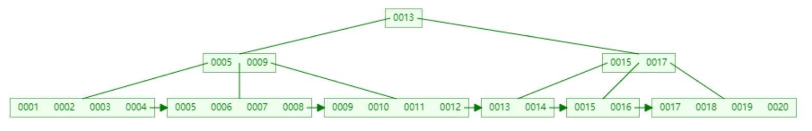
Complete Missing B+ Tree Operations

quick start

Header Page 存储布局

file type
page size
root page no
first leaf page no
first empty page no
schema size
stats size
schema
stats

Inner Page 存储布局

file type
page size
next page no (for empty page)
the number of pointers
first pointer

对于 key 和 pointer 的布局，可以参考

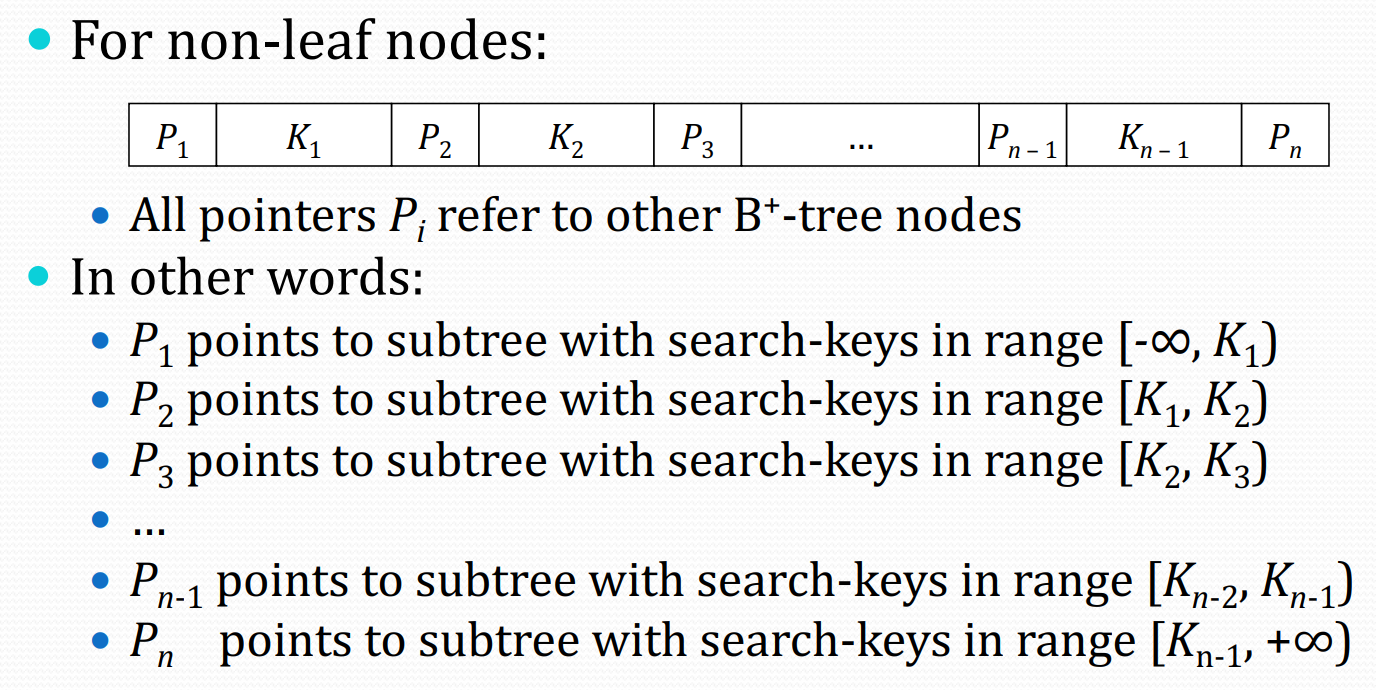
即对于一个 pointer 而言，左侧 ＜，右侧 ≥

Leaf Page 存储布局

file type
page size
next leaf page no (for leaf page) or next page no (for empty page)
the number of tuples
first tuple

tuple 有序排列，其内部布局仍由 PageTuple 管理

Leaf Page 和 Inner Page 均为 Data Page，且均可能成为 Root Page

对应的类从原始页中提取并缓存相关信息，使用 loadPageContents 进行同步

文件结构

.
├── BTreeFilePageTuple.java
├── BTreeFileVerifier.java
├── BTreePageTypes.java
├── BTreeTupleFile.java
├── BTreeTupleFileException.java
├── BTreeTupleFileManager.java
├── DataPage.java
├── FileOperations.java
├── HeaderPage.java
├── InnerPage.java
├── InnerPageOperations.java
├── LeafPage.java
├── LeafPageOperations.java
└── package.html

其中

BTreeTupleFile 在 file 级别下对 tuple 进行增删改查
BTreeTupleFileManager 用于创建和打开 tuple file
BTreeFilePageTuple 为 tuple 级别操作
BTreeFileVerifier 用于检查 B+ Tree 结构是否合法
FileOperations 用于获取和释放 data page
HeaderPage / InnerPage / LeafPage 定义了存储结构，完成一些单 page 的操作
InnerPageOperations / LeafPageOperations，完成一些跨 page 的操作

navigateToLeafPage

使用 List<Integer> 记录从 root page 到 leaf page 的所经过的所有 page no

使用 TupleComparator.comparePartialTuples 比较当前的 tuple 和 inner page 中的 key 即可

实现后，可以实现单 leaf page 的 B+ Tree

splitLeafAndAddTuple

需要分裂一个 leaf page 为两个，并插入一个 tuple

首先获取一个新的 data page，并初始化为 leaf page，然后进行 tuple 的迁移

需要考虑该 leaf page 是否存在 parent page

若不存在

该 leaf page 即为 root page

需要获取一个新的 data page，并初始化为 inner page，其初始的 key 就是新 leaf page 的第一个 tuple

由于是 moveTuplesRight

若存在

获取该 parent page，然后调用 InnerPageOperations.addTuple 即可

最后调用 addTupleToLeafPair 即可

实现后，可以实现最多一个 inner page (即 root page) 的 B+ Tree

movePointers

需要在两个 inner pages 之间迁移 entries (key, pointer)

相当 tricky，似乎并未完全正确实现

对应的方法在 InnerPage 中的 movePointersLeft 和 movePointersRight

先分析一下调用轨迹

首先是比较特殊的 movePointersRight，由于分裂 page 时都是向右迁移

对于 leaf page 和 inner page 都是如此

所以存在这样的一条调用轨迹

InnerPageOperations.addTuple

这个方法很关键，是向 inner page 中插入的入口方法

    public void addTuple(InnerPage page, List<Integer> pagePath,
                         int pagePtr1, Tuple key1, int pagePtr2) {

        // The new entry will be the key, plus 2 bytes for the page-pointer.
        int newEntrySize =
                PageTuple.getTupleStorageSize(tupleFile.getSchema(), key1) + 2;

        logger.debug(String.format("Adding new %d-byte entry to inner page %d",
                newEntrySize, page.getPageNo()));

        if (page.getFreeSpace() < newEntrySize) {
            logger.debug("Not enough room in inner page " + page.getPageNo() +
                    "; trying to relocate entries to make room");

            // Try to relocate entries from this inner page to either sibling,
            // or if that can't happen, split the inner page into two.
            if (!relocatePointersAndAddKey(page, pagePath,
                    pagePtr1, key1, pagePtr2, newEntrySize)) {
                logger.debug("Couldn't relocate enough entries to make room;" +
                        " splitting page " + page.getPageNo() + " instead");
                splitAndAddKey(page, pagePath, pagePtr1, key1, pagePtr2);
            }
        } else {
            // There is room in the leaf for the new key.  Add it there.
            page.addEntry(pagePtr1, key1, pagePtr2);
        }

    }

首先获取需要插入的 (key, pointer) 的大小

若该 inner page 空间足够，则直接插入

否则尝试与 sibling 进行 entries 的迁移，再进行插入

若仍失败，则需要分裂该 inner page，再进行插入

先观察 splitAndAddKey，其中会获取一个新的 data page，并初始化为 inner page (no entries)，然后判断原 inner page 是否存在 parent page

若不存在
- 调用 movePointersRight，其 parentKey 为 null
若存在
- 调用 movePointersRight，其 parentKey 为原 inner page 对应的 key

最后再进行一些处理

再观察 relocatePointersAndAddKey，其中会对 left sibling 和 right sibling 分别调用 tryNonLeafRelocateForSpace，得到可以迁移的空间

其算法如下

sibling 的剩余空间先减去 parentKey 的大小，因为在 movePointers 系列函数中，parentKey 会置入 sibling 中
然后按照顺序依次迁移原 inner page 的 (key, pointer) 对，直至双方的剩余空间都可以容纳刚开始需要插入的 (key, pointer)
- 这是因为原 (key, pointer) 本来应该插入在 inner page 中
- 但由于迁移，插入的位置可能迁移到了 sibling 中

其迁移的对数作为参数传入 movePointersLeft 和 movePointersRight 中

这便是在 insert 语义下 movePointers 的所有调用上下文

在 delete 语义下，其所有调用上下文在 deletePointer 中

下面分析具体的迁移过程

首先是 movePointersRight

若 parentKey 不为 null，以如下的 B+ Tree 为例

目前先无视阶数的影响

设参数 count = 2，则具体的迁移过程如下

这里需要考虑一些特殊情形

若 count = the number of keys
- 在这里就是 count = 3
- 那么就会留下一个单独的 pointer，不足以构成一个 inner page
- 直接报错处理
若 count = the number of pointers
- 在这里就是 count = 4
- 那么所有的 (key, pointer) 都迁移到了 sibling 中
- 此时就没有新的 parent key 提供给 parent page 了

若 parentKey 为 null，以如下的 B+ Tree 为例

设参数 count = 2，则具体的迁移过程如下

除了上述的特殊情形，还需要保证 count >= 2，否则无法初始化 inner page

然后是 movePointersLeft，根据上述调用上下文的分析，其参数 parentKey 不可能为 null

以如下的 B+ Tree 为例，设参数 count = 2，则具体的迁移过程如下

特殊情形在上面已经讨论过了

在实际的测试中

testBTreeTableThreeLevelInsert 会出现 buffer pool 溢出
- 考虑增加 nanodb.pagecache.size
- 具体的，修改 ServerProperties 类中的 DEFAULT_PAGECACHE_SIZE 字段
- 于是测试可以通过
- 对 B+ Tree 的层数进行估算
  - tuple 的平均大小为 1 + 4 + 200 = 205，需要插入 100000 个
  - 每个 leaf page 可以容纳 (8192 - 5) / 205 = 39
  - 设每个 inner page 可以容纳 x 个 key，则 (x + 1) * 2 + x * 205 <= 8192 - 5，得 x <= 39
  - 从而 B+ Tree 的层数为 $log_{39}(100000) = 4$
testBTreeTableMultiLevelInsertDelete 在 verify 时会出现 content 不一致
- 感觉框架代码中 delete 的实现存在问题，或者自己的理解有问题

Support for B+ Tree Indexes

对于索引的理解

an index is simply a table that is built against another table, containing a subset of the referenced table’s columns, and including an extra column that holds file-pointers to tuples in the referenced table
例如，对于如下的操作

CREATE TABLE t (
    a INTEGER,
    b VARCHAR(30),
    c FLOAT
);

CREATE INDEX i ON t (a);

会在 datafiles 文件夹中创建文件 t.tbl 和 t_i.idx

其中 t_i.idx 就是以 heapfile 为存储格式的 table，其 schema 如下

t.a : INTEGER, t.#TUPLE_PTR : file-pointer

添加索引功能，需要修改 PropertyRegistry.initProperties

”nanodb.enableIndexes” should be set to true to support indexes in the first place
”nanodb.createIndexesOnKeys” should be set to true to automatically create indexes on primary/unique/foreign keys

索引功能的实现主要依赖 RowEventListener 机制，IndexUpdater 实现了该接口，其中定义了 insert / update / delete 一个 tuple 前后应该执行的操作

EventDispatcher 类会注册 RowEventListener，并在合适的位置依次调用所有的 RowEventListener，注册的顺序即为调用的顺序

具体的位置如下

insert - InsertCommand
update - UpdateCommand
delete - DeleteCommand

可以回顾 lab1 中对于这些流程的分析

另外。EventDispatcher 类还会注册 CommandEventListener，并在 doCommand 中执行 command 前后调用所有的 CommandEventListener

对于 IndexUpdater 而言，目前的设计是

insert 后 / update 后，添加对应的索引
delete 前 / update 前，删除对应的索引

也就是索引的更新被拆分为了删除和添加操作

所以只需实现 addRowToIndexes 和 removeRowFromIndexes

具体可以参考 BasicIndexManager 中 populateIndex 的过程，核心数据结构是 IndexInfo，其中包含了

TableInfo
- tableName
- tupleFile - 存储表的文件
indexColRefs
- indexName
- colIndexes - 即 column 在对应 table schema 的索引集合
- constraint
tupleFile - 存储索引的文件

目前索引的类型包括 ordered index 和 hashed index，但由于 HashedTupleFile 尚无具体的实现，所以只能使用 ordered index，即利用上文实现的 BTreeTupleFile (SequentialTupleFile)

大概思路是

根据原始的 tuple 和 column refs，利用 IndexUtils.makeTableSearchKey 构造 index tuple
利用 IndexUtils.findTupleInIndex 判断该 index tuple 是否已经在索引文件中
- 由于内部 tuple 的比较模式是 IGNORE_LENGTH
- 所以即使 index tuple 不包含 external reference，也可以判断出来
使用 TupleFile 的 addTuple 和 deleteTuple 接口修改索引文件
- 注意在 BTreeTupleFile 的实现中，deleteTuple 要求参数 tuple 必须为 BTreeFilePageTuple
- 所以不能使用 IndexUtils.makeTableSearchKey 构造的 TupleLiteral
- 而应使用 findTupleInIndex 返回的 PageTuple

相关的测试用例在 TestIndexOps 中，不过存在一些 bug

Analysis of Implementation

Given NanoDB’s B+ tree implementation, consider a simple schema where an index is built against a single integer column:

 CREATE TABLE t (
     -- An index is automatically built on the id column by NanoDB.
     id INTEGER PRIMARY KEY,
     value VARCHAR(20)
 );

Answer the following questions.

A1.  What is the total size of the index's search-key for the primary-key
     index, in bytes?  Break down this size into its individual components;
     be as detailed as possible.  (You don't need to go lower than the
     byte-level in your answer, but you should show what each byte is a
     part of.)

以如下的插入语句为例

INSERT INTO t VALUES (1, 'abc')

对应的 index tuple 为 TL[1,FP[1:2]]，其大小为 9 bytes，由如下三部分组成

bitmap - 1 byte
integer - 4 bytes
file pointer (pageno + offset) - 4 bytes

A2.  What is the maximum number of search-keys that can be stored in leaf
     nodes of NanoDB's B+ tree implementation?  You should assume a page-
     size of 8192 bytes.

回顾 leaf page 的存储布局，第一个 tuple 在 offset = 5 处

所以最多可以容纳的 index tuple 的数量为 (8192 - 5) / 9 = 909

A3.  What is the maximum number of keys that can be stored in inner nodes
     of this particular implementation?  (Recall that every key must have
     a page-pointer on either side of the key.)

每一个 pointer 的大小为 2 bytes，第一个 pointer 在 offset = 5 处

设最多可以容纳的 index tuple 的数量为 x，则有关系

9 * x + 2 * (x + 1) <= 8192 - 5

得到 x <= 744，即最多可以容纳的 index tuple 的数量为 744

A4.  In this implementation, leaf nodes do not reference the previous
     leaf, only the next leaf.  When splitting a leaf into two leaves,
     what is the maximum number of leaf nodes that must be read or written,
     in order to properly manage the next-leaf pointers?

     If leaves also contained a previous-leaf pointer, what would the
     answer be instead?

     Make sure to explain your answers.

两读两写

int nextPageNo = leaf.getNextPageNo();
leaf.setNextPageNo(newLeaf.getPageNo());
newLeaf.setNextPageNo(nextPageNo);

对于 prev-leaf pointer 同理

A5.  In this implementation, nodes do not store a page-pointer to their
     parent node.  This makes the update process somewhat complicated, as
     we must save the sequence of page-numbers we traverse as we navigate
     from root to leaf.  If a node must be split, or if entries are to be
     relocated from a node to its siblings, the node’s parent-node must
     be retrieved, and the parent’s contents must be scanned to determine
     the node’s sibling(s).

     Consider an alternate B+ tree implementation in which every node
     stores a page-pointer to the node’s parent.  In the case of splitting
     an inner node, what performance-related differences are there between
     this alternate representation and the given implementation, where
     nodes do not record their parents?  Which one would you recommend?
     Justify your answer.

对于现有的实现，关注 InnerPage 的 splitAndAddKey 方法，之前分析了一部分

获取一个新的 data page，并初始化为 inner page (no entries)
判断原 inner page 是否存在 parent page，并合理的调用 movePointersRight
将新的 (key, pointer) 插入到 inner page 中
根据 page path 判断是否存在 parent page
- 若存在，修改 page path，并对 parent page 递归调用 addTuple
- 若不存在，获取一个新的 data page，并初始化为 inner page，并修改 header page 的 root page no

若每一个 data page 都存在指向自己 parent page 的 pointer，那么就不需要 page path，直接根据存储的信息获取 parent page，具体的

若存在 parent page，直接对 parent page 递归调用 addTuple
若不存在，获取一个新的 data page，并初始化为 inner page，同时设置之前新 inner page 的 parent page no 信息，并修改 header page 的 root page no

对于现有的实现，在每次插入和删除 tuple 时，都需要在 navigation 的同时获取 page path 信息，实际上开销并不算大，但这减少了 data page 之间的耦合，data page 之间仅通过 tuple key 关联在一起，在优化结构时，例如需要大规模移动 page 修改 page no，就不需要对 B+ Tree 内部进行任何修改

A6.  It should be obvious how indexes can be used to enforce primary keys,
     but what role might they play with foreign keys?  For example, given
     this schema:

     CREATE TABLE t1 (
         id INTEGER PRIMARY KEY
     );
     CREATE TABLE t2 (
         id INTEGER REFERENCES t1
     );

     Why might we want to build an index on t2.id?

首先了解一下 nanodb 中的 constraint 类型

NOT NULL
UNIQUE
PRIMARY KEY
FOREIGN KEY

这些 constraints 由 DatabaseConstraintEnforcer 监测，其实现了 RowEventListener 接口

具体的创建在 CreateTableCommand 的 initTableConstraints 方法中

primary key 和 unique key 会有对应的 KeyColumnRefs

即作为 candidate key

primary key 还会被施以 not null

对于 foreign key 而言，一些细节如下

若未指定 reference 的具体字段，则默认为 reference table 的 PRIMARY KEY
- 标准格式为 id INTEGER REFERENCES t1 (id)
需要检查 reference 的字段是否为 candidate key
构造对应的 ForeignKeyColumnRefs
需要修改 reference table 中 schema 的 referencingTables

对于向外键建立索引的原因，可以参考 Why do foreign keys need to be indexed? - Katastros，总结为

Only when the unique key or primary key is not updated or deleted, there is no need to create an index for the foreign key. Creating an index for the foreign key of a child table can have two benefits:

To avoid table locks on the child table, instead, the database will acquire row locks on the index.
Avoid full table scans on sub-tables. Assume that the records of the department main table with id=10 are deleted. If the department_id foreign key of the employees sub-table does not have an index, then the entire table scans the employees sub-table to confirm whether there are records with department id=10.

A7.  Over time, a B+ tree's pages, its leaf pages in particular, may become
     severely out of order, causing a significant number of seeks as the
     leaves are traversed in sequence.  Additionally, some of the blocks
     within the B+ tree file may be empty.

     An easy mechanism for regenerating a B+ tree file is to traverse the file's
     tuples in sequential order (i.e. from the leftmost leaf page, through
     all leaf pages in the file), adding each tuple to a new B+ tree file.
     The new file may then replace the old file.

     Imagine that this operation is performed on a B+ tree file containing
     many records, where all records are the same size.  On average, how full
     will the leaf pages in the newly generated file be?  You can state your
     answer as a percentage, e.g. "0% full".  Explain your answer.

回顾 B+ Tree 的半满特性，对于 $n$ 阶 B+ Tree

inner page 至少应包含 $\lceil \frac{n}{2} \rceil$ 个 pointers，至多应包含 $n$ 个 pointers
leaf page 至少应包含 $\lceil \frac{n-1}{2} \rceil$ 个 tuples，至多应包含 $n$ 个 tuples

例如，对于 5 阶 B+ Tree，顺序插入 1 ~ 16 后的结果如下

可以发现左侧的 leaf page 都处于半满的状态

所以实际的利用率趋近于 $\frac{\lceil \frac{n-1}{2} \rceil}{n}$

更多的讨论可以参考 InnoDB B-tree 顺序插入优化及问题

A8.  Consider a variation of the approach in A7:  Instead of making one pass
     through the initial B+ tree file, two passes are made.  On the first pass,
     the 1st, 3rd, 5th, 7th, ... tuples are added to the new file.  Then, on the
     second pass, the 2nd, 4th, 6th, 8th, ... tuples are added to the new file.
     On average, how full will the leaf pages in the newly generated file be?
     Explain your answer.

例如，对于 5 阶 B+ Tree，依次插入 1 / 3 / 5 / ... / 19 / 2 / 4 / 6 / ... / 20 后的结果如下

具体的形态和阶数相关，显然利用率会更高

Deletion Analysis

之前只分析了 insert 的原理，delete 的原理更加复杂，先挖个坑 🤣

Extra Credit

pin and unpin
optimize
analyze

类似 lab3 中的 statistics collection，只是获取 tuple 的方式有所变化

目前只统计 leaf page 的数量作为 numDataPages

还需要实现 BTreeTupleFileManager 中的 saveMetadata 方法，直接照抄即可

CREATE TABLE bt (
    a INTEGER,
    b VARCHAR(20)
) PROPERTIES (storage = 'btree');

INSERT INTO bt VALUES (1, 'abc');
INSERT INTO bt VALUES (2, 'xyz');
INSERT INTO bt VALUES (1, 'def');

ANALYZE bt;

show table bt stats;

index scan node

由于在 planner 中利用 index scan node，需要对 predicate 进行更细致的处理

所以只考虑在 makeSimpleSelect 中使用 index scan node，需要修改其返回值为 PlanNode 类型

因为 IndexScanNode 并非 SelectNode 的子类

另外，测试时需要将 planner 设置为 SimplestPlanner

下面分析一下流程

需要使用 AnalyzedPredicate 类分析 predicate，得到 rangeConjuncts
- rangeConjuncts 要求形式均为 column op value，是同一个 column，且能构成一个范围
- 例如 a > 5 AND a <= 10 就是一个 rangeConjuncts
AnalyzedPredicate 内部提供了 canUseIndex 方法，根据 index 和 rangeConjuncts 生成 IndexScanEndpoints
- 该方法首先定位有 index 的 column，得到对应的 rangeConjuncts
- 使用这些 rangeConjuncts 构造 IndexScanEndpoints，主要工作是合并 conjuncts 和生成边界 value
最后使用 IndexInfo 和 IndexScanEndpoints 构造 IndexScanNode

IndexScanNode 在实际执行中，会根据 startLookupValue 和 startPredicate，在 index tuple file 中定位到第一个满足条件的 index-tuple，并根据其 file pointer，在 table tuple file 得到真正的 tuple，之后的 next 操作只需考虑 endPredicate 即可

实际上框架代码存在一些 bug，例如若 startPredicate 为 id >= 144，而实际的 tuple file 中并不存在 id = 144 的 tuple，那么就无法正确定位到第一个满足条件的 index-tuple，因为框架代码只使用了 findFirstTupleEquals(startLookupValue)

SequentialTupleFile 尚可以 fix，HashedTupleFile 就无能为力了

最后的任务就是建立 IndexScanNode 的 costing model，大部分类似 FileScanNode，除了

选择率的计算需要考虑区间
cpuCost 可以直接置为最终乘上选择率的 numTuples，因为不必 eval predicate，即 perRowCost 为 1，且不必完全遍历

lab7

对应的课件

算法参考

一文讲懂 ARIES Recovery 算法 - hhwyt

Step 1: Enable Transaction Processing in NanoDB

需要修改 PropertyRegistry.initProperties，添加事务功能

”nanodb.enableTransactions” should be set to true to turn on transaction processing
”nanodb.flushAfterCmd” should be changed to false so that the buffer pool is no longer flushed after every command

同时禁用索引功能

目前 index 和 DDL 均不支持事务

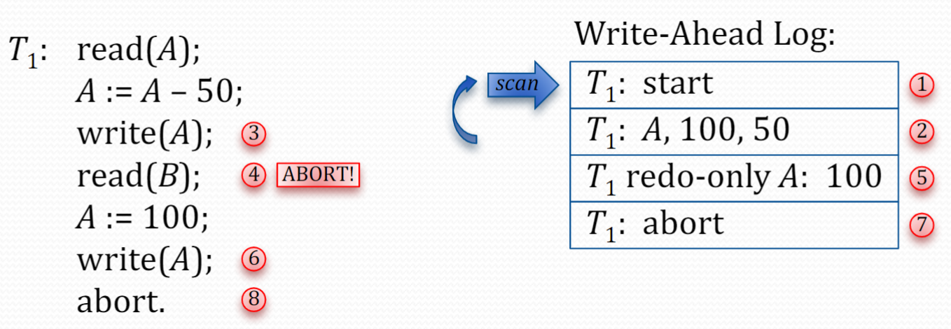
Step 2: Add Logging to Heap Tuple Files

在合适的位置调用 storageManager.logDBPageWrite，以记录 heap tuple file 的修改

目前的考虑是

HeapTupleFile 中的 addTuple / updateTuple / deleteTuple
HeapTupleFileManager 中的 saveMetadata (header page)

Step 3: Implement an Atomic Force-WAL Operation

基本工作就是将 txnStateNextLSN 至参数 lsn 之间的 WAL 落盘

可能存在多个 WAL files，这导致同步可能不是原子的

当所有的 WAL files 落盘后，才会修改 txnStateNextLSN，这是 transaction state 的一部分

考虑在同步过程中 crash，由于 WAL page 并不支持事务，所以会丢失一部分 WAL

In general, data pages relating to the write-ahead log are not transacted. (It wouldn’t make sense to log changes to write-ahead log pages in the write-ahead log.)

这个问题尚未得到合理的解决

Step 4: Enforce the Write-Ahead Logging Rule

Before a dirty table-page is flushed to disk, must ensure that all logs pertaining to that page have been sync’d to disk.

为此需要在 BufferManager.writeDirtyPages 中，添加相关的代码以遵循上述规则

框架代码抽象出了一个接口 BufferManagerObserver，TransactionManager 实现了该接口

思路就是遍历所有的 dirty pages，然后获取其中类型为 HEAP_TUPLE_FILE 和 BTREE_TUPLE_FILE 的 LSN

只有这两种 data pages 是 transacted 的

以其中最大的 LSN 为参数调用 forceWAL 即可

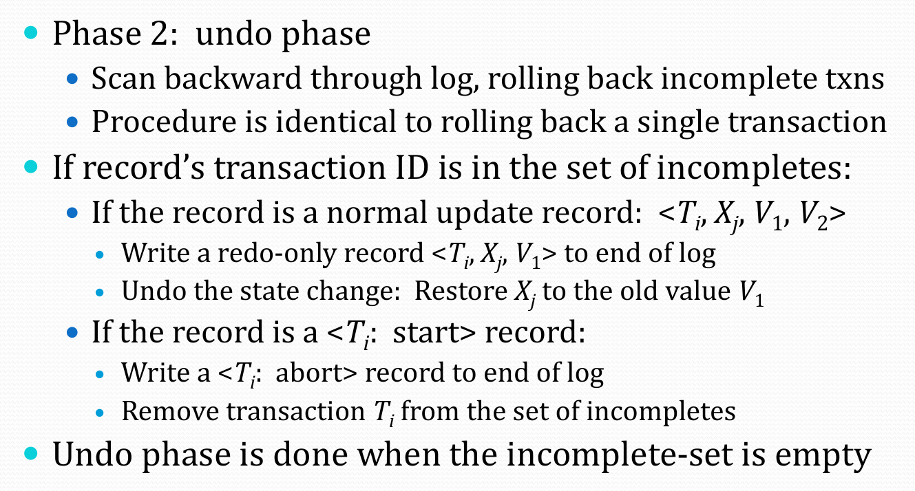
Step 5: Implement Transaction Rollback

主要内容是实现 rollback 功能

流程可以参考

由于每个 WAL record (except START) 都包含 PrevLSN 字段，所以反向遍历效率很高

具体的 record 布局可以参考 edu.caltech.nanodb.storage.writeahead，此处不再赘述

有两个辅助函数完成了核心工作

applyUndoAndGenRedoOnlyData
- 将 undo data (old version of the data) 应用到 page 中
- 并根据 undo data 生成 redo-only update record 的 data segments
  - 注意这里 redo-only 的含义是仅在 redo 阶段考虑的 record
writeRedoOnlyUpdatePageRecord
- 写入 redo-only update record
- 实际上写入的就是 update record 中的 undo data

注意区分 WALManager 中的 nextLSN 字段和 TransactionState 中的 lastLSN 字段，在同步的情形下 lastLSN 即为 nextLSN 的前一个 LSN

另外也需要区分 WALManager 中的 nextLSN 字段和持久化在 txnstate.dat 中的 nextLSN 字段，在 WAL 没有落盘的情况下，前者有可能大于后者

Step 6: Implement Redo and Undo Processing

Redo Processing

流程可以参考

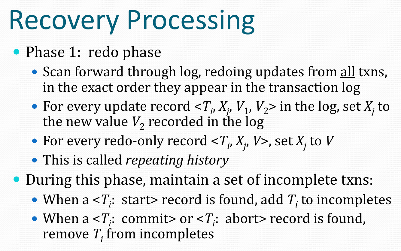
使用辅助函数 applyRedo 将 redo data (new version of the data) 应用到 page 中

有两个要点

及时移动 walReader 的 offset
使用 currLSN 及时更新 transactionID 对应的 recoveryInfo，这在后面的 undo process 中会使用到

Undo Processing

流程可以参考

思路类似 rollbackTransaction，有两处不同

不考虑 UPDATE_PAGE_REDO_ONLY 类型的 record
在写入新的 record 时，使用的 transactionID 和 prevLSN 需要从 recoveryInfo 中获得

简单的分析一下流程

从 nextLSN 开始反向遍历
1. 当遇到跨 file 的情形时，利用 OFFSET_PREV_FILE_END 字段
获取每个 record 的 transactionID
若该 transactionID 属于 incompletes，则根据 record 类型进行处理
1. UPDATE_PAGE - 需要写入一个 UPDATE_PAGE_REDO_ONLY 类型的 record，其 prevLSN 为该 txn 的 lastLSN，由于 WAL 中可能存在多个 txn 交错的情形，所以需要显式的记录，在写入完成后，还需要更新该 txn 的 lastLSN
2. START_TXN - 不再赘述

txn 交错的情形可以参考下图

Step 7: Testing

schemas/writeahead/basic-tests.sql 中有一些基础的测试用例

其中 2B 和 2C 完全相同

参考实验指南，以相同形式给出如下测试用例

-- TODO:  INIT

CRASH;

-- TODO:  RESTART NANODB

-- TODO:  INIT

CREATE TABLE testwal (
  a INTEGER,
  b VARCHAR(30),
  c FLOAT
);

INSERT INTO testwal VALUES (1, 'abc', 1.2);
INSERT INTO testwal VALUES (2, 'defghi', -3.6);

SELECT * FROM testwal;  -- Should list both records

CRASH;

-- TODO:  RESTART NANODB

SELECT * FROM testwal;  -- Should list both records

CRASH;

-- TODO:  RESTART NANODB

-- TODO:  INIT

CREATE TABLE testwal (
  a INTEGER,
  b VARCHAR(30),
  c FLOAT
);

BEGIN;

INSERT INTO testwal VALUES (1, 'abc', 1.2);
INSERT INTO testwal VALUES (2, 'defghi', -3.6);

SELECT * FROM testwal;  -- Should list both records

COMMIT;

SELECT * FROM testwal;  -- Should list both records

CRASH;

-- TODO:  RESTART NANODB

SELECT * FROM testwal;  -- Should list both records

CRASH;

-- TODO:  RESTART NANODB

-- TODO:  INIT

CREATE TABLE testwal (
  a INTEGER,
  b VARCHAR(30),
  c FLOAT
);

INSERT INTO testwal VALUES (1, 'abc', 1.2);

BEGIN;

INSERT INTO testwal VALUES (2, 'defghi', -3.6);

SELECT * FROM testwal;

ROLLBACK;

SELECT * FROM testwal;

CRASH;

-- TODO:  RESTART NANODB

SELECT * FROM testwal;

CRASH;

-- TODO:  RESTART NANODB

-- TODO:  INIT

CREATE TABLE testwal (
  a INTEGER,
  b VARCHAR(30),
  c FLOAT
);

INSERT INTO testwal VALUES (1, 'abc', 1.2);

BEGIN;

INSERT INTO testwal VALUES (2, 'defghi', -3.6);

SELECT * FROM testwal;

-- FLUSH;
CRASH;

-- TODO:  RESTART NANODB

SELECT * FROM testwal;

CRASH;

-- TODO:  RESTART NANODB

-- TODO:  INIT

CREATE TABLE testwal (
  a INTEGER,
  b VARCHAR(30),
  c FLOAT
);

BEGIN;
INSERT INTO testwal VALUES (1, 'abc', 1.2);
COMMIT;

BEGIN;
INSERT INTO testwal VALUES (2, 'defghi', -3.6);
ROLLBACK;

BEGIN;
INSERT INTO testwal VALUES (-1, 'zxywvu', 78.2);
COMMIT;

CRASH;

-- TODO:  RESTART NANODB

SELECT * FROM testwal;
CRASH;

-- TODO:  RESTART NANODB

-- TODO:  INIT

CREATE TABLE testwal (
  a INTEGER,
  b VARCHAR(30),
  c FLOAT
);

BEGIN;
INSERT INTO testwal VALUES (1, 'abc', 1.2);
COMMIT;

BEGIN;
INSERT INTO testwal VALUES (2, 'defghi', -3.6);
ROLLBACK;

BEGIN;
INSERT INTO testwal VALUES (-1, 'zxywvu', 78.2);
ROLLBACK;

CRASH;

-- TODO:  RESTART NANODB

SELECT * FROM testwal;
CRASH;

-- TODO:  RESTART NANODB

将测试点归类如下

显式和隐式 txn
rollback
txn 未结束之前 crash
- crash 之前 flush，从而测试 recovery 过程是否能够处理不完整的 txn
多次 restart，验证后续的 restart 为 no-op

另外，在测试中发现了一个问题，由于关闭了 flushAfterCmd，对于每条 insert 语句，实际上落盘的是对应的 WAL，而非具体的数据

当 restart 时，会在 recovery 过程 redo 这些 update record，即写入对应的 data page

然而这里的写入并不会给对应的 data page 设置 pageLSN

回忆之前 insert 设置的 pageLSN 作为非持久化数据，在 restart 后已经丢失

又因为这些 data page 已经 dirty 了，所以在 beforeWriteDirtyPages 中会出现 HEAP_TUPLE_FILE 或 BTREE_TUPLE_FILE 缺失 LSN 的情形

所以考虑将 throw exception 降级为 log warning

Analysis

这里为了配合 ARIES Recovery 算法，buffer pool 的策略是 STEAL / NO-FORCE，即

允许将未提交事务的改动刷盘
不要求在事务提交时把该事务的所有改动刷盘

前者在代码中的体现较少，后者的一个例子就是上面测试中发现的问题，即已经 commit 了，但是数据并未落盘，而是在重启后 recovery 的过程落盘

下面分析一下 WAL 协议在代码中的体现，即

必须保证所有 page 刷盘之前与它有关的所有 log 已经刷盘
必须保证事务提交前该事务的所有 log 已经刷盘

对于前者，data page 存在 pageLSN 字段，在 writeUpdatePageRecord 和 writeRedoOnlyUpdatePageRecord 中均会设置该字段，而在 beforeWriteDirtyPages 中会根据该字段调用 forceWAL

在设置该字段后，总是会调用对应 page 的 syncOldPageData 方法，以保证每个 record reflects the changes since the previous “update” record

对于后者，在 commitTransaction 中，会以内存中的 nextLSN 为参数调用 forceWAL

另外一个值得注意的点是 record 的跨 file 问题，LSN 的计算是通过 computeNextLSN 完成的，当 offset 超出阈值时，就会切换到下一个 WAL，实际上存储的内容已经超出了阈值，但可以保证最后一个 record 总是完整的

Challenges

前置条件是 lab 1.3，即优化存储性能

对应的数据集为 TPC-H Homepage

NanoDB Assignments

TOC

info

intro

lab1

NanoDB Tuple Updates and Deletion

NanoDB Buffer Management

NanoDB Storage Performance

lab2

overview

features

paradigm

note

Projection

No FROM clause

FROM clause subqueries

FROM clause join

ORDER BY clauses

Grouping and Aggregation

LIMIT and OFFSET clauses

lab3

Statistics Collection

Plan Costing

ProjectNode

RenameNode

SortNode

HashedGroupAggregateNode

FileScanNode

SimpleFilterNode

NestedLoopJoinNode

Estimating Selectivity

Estimating Plan-Node Column Statistics

Testing Plan Costing

Basic Plan Costs

Costing Joins

Updating Column Statistics

Extra Credit

lab4

overview

implementation

test

lab5

Planning Subqueries

Costing Expressions with Subqueries

Correlated Evaluation

Test

Extra Credit

lab6

Complete Missing B+ Tree Operations

quick start

navigateToLeafPage

splitLeafAndAddTuple

movePointers

Support for B+ Tree Indexes

Analysis of Implementation

Deletion Analysis

Extra Credit

lab7

Step 1: Enable Transaction Processing in NanoDB

Step 2: Add Logging to Heap Tuple Files

Step 3: Implement an Atomic Force-WAL Operation

Step 4: Enforce the Write-Ahead Logging Rule

Step 5: Implement Transaction Rollback

Step 6: Implement Redo and Undo Processing

Redo Processing

Undo Processing

Step 7: Testing

Analysis

Challenges

No `FROM` clause

`FROM` clause subqueries

`FROM` clause join

`ORDER BY` clauses

`LIMIT` and `OFFSET` clauses