Info

https://hongjin-liang.github.io/teaching/concurrency/index.html

Overview

Concurrent Program

A concurrent program = concurrent objects + their clients

concurrent objects 可以是一个 mutex，也可以是一个并发数据结构

client 只能通过调用 concurrent objects 的接口访问共享内存

多个 client 会并发的访问 concurrent objects，因而会产生不确定的交错访问

Memory Models

下面介绍内存模型，若硬件能够提供源代码级别程序的交错访问，那么被称为 Sequential Consistency

interleaving semantics

然而

No muticore processor implements SC
Compiler optimizations invalidate SC

每一种硬件架构都会提供自己的弱内存模型，例如

和

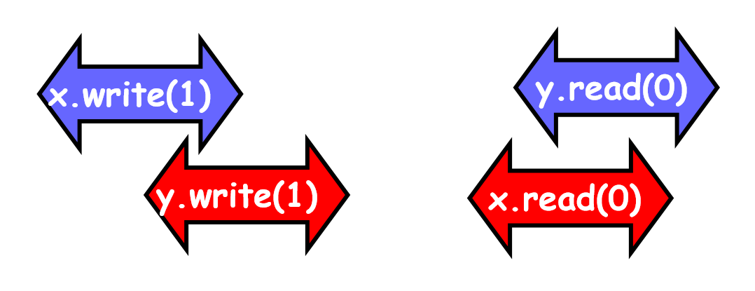
这就会带来一些问题，例如 Store buffering (SB)

考虑如下一段程序

Initially:  x = y = 0

// thread 1
x = 1;
r1 = y;

// thread 2
y = 1;
r2 = x;

在 x86-TSO memory model 下，可能会出现 r1 = r2 = 0，也就是数据只写入了 buffer，还未写入共享内存，这种情形在 SC 下是不可能发生的

在编译优化下，还可能出现指令乱序，例如 thread 1 的 r1 = y; 在 x = 1; 之前执行，同样也会导致 r1 = r2 = 0

另一个例子是 Load buffering (LB)

Initially:  x = y = 0

// thread 1
r1 = x;
y = 1;

// thread 2
r2 = y;
x = 1;

可能会出现 r1 = r2 = 1，也就是读操作被延迟了

在这样的环境下，高级语言的程序员需要考虑硬件架构，又要考虑编译优化，实在是太困难了

于是，硬件设计者和编译器设计者约定，只要程序具有 DRF 的性质，那么就可以保证程序的执行是 SC 的，所以对于 client 端，并不需要考虑内存模型

然而，concurrent objects 端为了提高性能，在实现 concurrent algorithms 时，可能并不需要 SC，所以需要考虑内存模型

Course Overview

Weak memory models
- HMM (the core of Java memory model)
- TSO
- C11
Concurrent objects
- Linearizability
- Algorithms
  - Peterson Lock, Filter Lock, Lamport’s Bakery Lock
  - TAS Lock, Queue Locks
  - List-Based Sets
  - Concurrent Queues and Stacks

Memory Models

Design Criteria

DRF programs have the same behaviors as in SC model

需要定义何为 DRF - A data race occurs when we have two concurrent conflicting operations

conflicting - 两个操作同时访问同一块内存，其中至少有一个是写操作
concurrent - 在不同的内存模型下有不同的定义
- 在 Java 中，定义为两个操作无法被 happens-before 关系排序
- 在 SC 下，happens-before 可以是 program-order，即每个线程自己的代码顺序，也可以是 synchronizes-with，即多线程之间使用同步原语
- 形式化的，在 SC 下， $\text{happens-before} = (\text{PO} \cup \text{SW})^{+}$ ，即传递闭包

Not too strong

要支持主流的编译优化

要支持主流硬件架构的 compilation schemes

Not too weak

保证类型安全和一些安全性保证

Happens-Before Memory Model (HMM)

上面提过，Happens-Before Order 就是 program-order 和 synchronizes-with 并集的传递闭包

在这样的内存模型下，read 可见的 write 如下

the most recent write that happens-before it
a write that has no happens-before relation

例如 r 读取的值可能是 w1 写入的，也可能是 w2 写入的

good speculation

对于之前的例子

Initially:  x = y = 0

// thread 1
x = 1;
r1 = y;

// thread 2
y = 1;
r2 = x;

是否可能出现 r1 = r2 = 0，根据 Happens-Before Order 建模

flowchart LR A["x = 0, y = 0"] --> B["x = 1"] A --> C["y = 1"] B --> D["r1 = y(0) - speculation"] C --> E["r2 = x(0) - speculation"] A -.-> D A -.-> E

虚线代表了 read 可能读取的 write 的来源，都是 no happens-before，所以是可能的

bad speculation

但是，在 HMM 下，可能出现 Out-of-Thin-Air Read，即凭空的 read

考虑如下的例子

Initially:  x = y = 0

// thread 1
r1 = x;
y = r1;

// thread 2
r2 = y;
x = r2;

是否可能出现 r1 = r2 = 42，根据 Happens-Before Order 建模

flowchart LR A["x = 0, y = 0"] --> B["r1 = x(42) - speculation"] A --> C["r2 = y(42) - speculation"] B --> D["y = r1(42) - accord to po"] C --> E["x = r2(42) - accord to po"] E -.-> B D -.-> C

注意这里是先对结果进行 speculation，然后根据 Happens-Before Order 得到其他的值，最终判断结果值的来源

虚线代表了 read 可能读取的 write 的来源，都是 no happens-before，所以是可能的

这就有可能破坏安全性保证

JMM

以 HMM 为核心，试图区分 good speculation 和 bad speculation，却引入了更多的问题

http://www.cs.umd.edu/~pugh/java/memoryModel/

Operational Semantics

Basic domains

Registers (local variables)

r ∈ Reg

Locations

x ∈ Loc

Values including 0

v ∈ Val

Thread identifiers

i ∈ Tid = {1, ... ,N}

Expressions and commands

e ::= r | v | e + e | ...
c ::= skip | if e then c else c | while e do c | c ; c | r := e | r := x | x := e | r := FAA(x, e) | r := CAS(x, e, e) | fence

这里区分了 x 和 e，对 x 的读写需要访问内存

Programs

P : Tid → Cmd

written as

P = c1 ∥ ... ∥ cN

The thread subsystem

Store

s : Reg → Val

s 代表寄存器的集合

State

⟨c, s⟩ ∈ Command × Store

Transitions

\overline{\text { skip; } c, s \stackrel{\varepsilon}{\rightarrow} c, s}

skip 指令直接跳过，此处 $\varepsilon$ 表示无需与内存子系统进行交互

\frac{c_1, s \stackrel{I}{\rightarrow} c_1^{\prime}, s^{\prime}}{c_1 ; c_2, s \stackrel{I}{\rightarrow} c_1^{\prime} ; c_2, s^{\prime}}

定义 ; 的语义，此处 $I$ 代表线程子系统和内存子系统的一次交互，例如 $R,W,U,F$

\frac{s^{\prime}=s[r \mapsto s(e)]}{r:=e, s \stackrel{\varepsilon}{\rightarrow} \text { skip, } s^{\prime}}

此处 $s[r \mapsto s(e)]$ 表示单点修改寄存器 $r$ 的值， $s(e)$ 表示通过寄存器计算 $e$ 的值

\frac{I=R(x, v)}{r:=x, s \stackrel{I}{\rightarrow} \operatorname{skip}, s[r \mapsto v]}

通过内存子系统读取内存 $x$ 的值到变量 $v$ 中，并修改寄存器 $r$ 的值

\frac{I=W(x, s(e))}{x:=e, s \stackrel{I}{\rightarrow} \text { skip, } s}

通过内存子系统将 $e$ 的值写入内存 $x$ 中

\begin{array}{l} \frac{s(e) \neq 0}{\text{if } e \text{ then } c_1 \text{ else } c_2, s \stackrel{\varepsilon}{\rightarrow} c_1, s} \newline \frac{s(e) = 0}{\text{if } e \text{ then } c_1 \text{ else } c_2, s \stackrel{\varepsilon}{\rightarrow} c_2, s} \newline \frac{}{\text { while } e \text { do } c, s \stackrel{\varepsilon}{\rightarrow} \text { if } e \text { then }(c ; \text { while } e \text { do } c) \text { else skip, } s} \end{array}

分支和循环语句，将循环递归转换为分支

\frac{I=U(x, v, v+s(e))}{r:=\mathbf{FAA}(x, e), s \stackrel{I}{\rightarrow} \text { skip, } s[r \mapsto v]}

Fetch-and-add，语义是将读取内存 $x$ 的值到寄存器 $r$ 中，并增加内存 $x$ 的值，此处引入了新的记号 $U$ ，代表原子读写内存

\begin{array}{l} \frac{I=R(x, v) \quad v \neq s(e_r)}{r:=\mathbf{CAS}\left(x, e_r, e_w\right), s \stackrel{I}{\rightarrow} \text { skip, } s[r \mapsto 0]} \newline \frac{I=U(x, v, s(e_w)) \quad v = s(e_r)}{r:=\mathbf{CAS}\left(x, e_r, e_w\right), s \stackrel{I}{\rightarrow} \text { skip, } s[r \mapsto 1]} \end{array}

Compare-and-swap，语义是将读取内存 $x$ 的值到变量 $v$ 中，若值和 $e_r$ 不等，则置寄存器 $r$ 为 $0$ ，否则置寄存器 $r$ 为 $1$ ，同时修改内存 $x$ 的值

注意这里两个对 storage subsystem 的交互是不同的，在后面 TSO storage subsystem 中会有所体现

\frac{}{\text { fence, } s \stackrel{F}{\rightarrow} \text { skip, } s}

最后是 fence 指令，使用 $F$ 强制内存读写

参考 The Art of Multiprocessor Programming Chapter 5，若不存在 FAA 或 CAS 指令，某些 current objects 是无法实现的

SC storage subsystem

对内存的读写对所有的线程即时可见

Machine state

M : Loc → Val

Transitions

\frac{I=W(x, v)}{M \stackrel{i: I}{\longrightarrow} M[x \mapsto v]}

此处 $i:I$ 表示线程 $i$ 对内存的修改

\frac{I=R(x, v) \quad M(x)=v}{M \stackrel{i: I}{\rightarrow} M}

读不修改内存

\frac{I=U\left(x, v_r, v_w\right) \quad M(x)=v_r}{M \stackrel{i: I}{\rightarrow} M\left[x \mapsto v_w\right]}

读内存并且修改

\frac{I=F}{M \stackrel{i: I}{\rightarrow} M}

fence 指令所带来的操作是 no-op

Lifting to concurrent programs

State

⟨P, S⟩ ∈ (Tid → Cmd) × (Tid → Store)

每个 tid 对应一个 cmd 和 store

Transition

\frac{P(i), S(i) \stackrel{I}{\rightarrow} c, s}{P, S \stackrel{i: I}{\longrightarrow} P[i \mapsto c], S[i \mapsto s]}

实际上定义了每个 thread 对 cmd 和 store 的修改在全局视角下的表示

Linking the thread and storage subsystems

综合 $P,S,M$

Transition

不访问内存的情形下，有

\frac{P, S \stackrel{i: \varepsilon}{\longrightarrow} P^{\prime}, S^{\prime}}{P, S, M \Rightarrow P^{\prime}, S^{\prime}, M}

访问内存的情形下，有

\frac{P, S \stackrel{i: I}{\rightarrow} P^{\prime}, S^{\prime} \quad M \stackrel{i: I}{\rightarrow} M^{\prime}}{P, S, M \Rightarrow P^{\prime}, S^{\prime}, M^{\prime}}

Allowed outcome

An outcome is a function

O : Tid → Store

An outcome O is allowed for a program P under SC if there exists M such that

P, S0, M0 =>∗ skip ∥ ... ∥ skip, O, M

定义了在 SC 内存模型下，所有线程寄存器的状态的可能结果

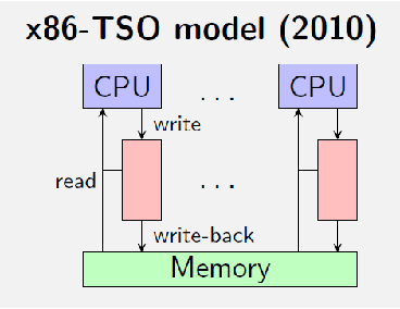
TSO storage subsystem

每个 thread 有一个 store buffer

所以内存的 Machine state 需要增加

A function B : Tid → (Loc × Val)∗

例如

thread #1 -> ((x, 1), (y, 2), (x, 3))

注意 store buffer 中的顺序是关键的

由此可以定义如下 transitions

write 交互不会修改内存，只会在 store buffer 的结尾添加对应的写操作
一次 propagate 操作会取出 store buffer 开头的写操作，并实际修改内存，thread subsystem 不会显式使用该交互
read 交互则将 store buffer 的写操作按顺序假装应用到内存中，由此进行读操作，但实际上并不会修改内存
RMW 代表 read modify write，注意该 transition 的前提是 store buffer 为空，也就是在执行该 transition 前，会隐式执行 propagate 操作，fence 交互同理
- 例如，对于 CAS 操作，若值不相等，则仅会进行 read 交互，而不会执行 RMW 交互，也就不会清空 store buffer

PSO storage subsystem

PSO 内存系统比 TSO 更弱，体现在 store buffer 对于不同变量的写可以乱序，例如，对于如下写操作

x = 1
y = 2
x = 3

store buffer 可以为

(x, 1), (x, 3), (y, 2)

也可以为

(y, 2), (x, 1), (x, 3)

为此，需要修改 write transition

\frac{I=W(x, v) \quad B(i) = b_1 \cdot b_2 \quad x \notin b_1}{M, B \stackrel{i: I}{\longrightarrow} M, B[i \mapsto b_1 \cdot \langle x, v\rangle \cdot b_2]}

添加 store-store-fence 交互

\frac{I = SSF}{M, B \stackrel{i: I}{\longrightarrow} M, B[i \mapsto \text{SSF} \cdot B(i)]}

实际上是在 store buffer 中添加一个标签 $\text{SSF}$

略微修改 write transition 即可

\frac{I=W(x, v) \quad B(i) = b_1 \cdot b_2 \quad x \notin b_1 \quad \text{SSF} \notin b_1}{M, B \stackrel{i: I}{\longrightarrow} M, B[i \mapsto b_1 \cdot \langle x, v\rangle \cdot b_2]}

Declarative Semantics

换种方式写笔记

这种定义语义的思想在之前 HMM 中已经有所体现，这一节将其形式化

Executions

Events 是图中的顶点，Relations 则是图中的边

rf 感觉就是对同一个内存地址所读取的值的 speculation

此处形式化定义 Event，i ∈ Tid ∪ {0} 中并上 0 是为了表示程序的初始状态，例如 x = 0, y = 0

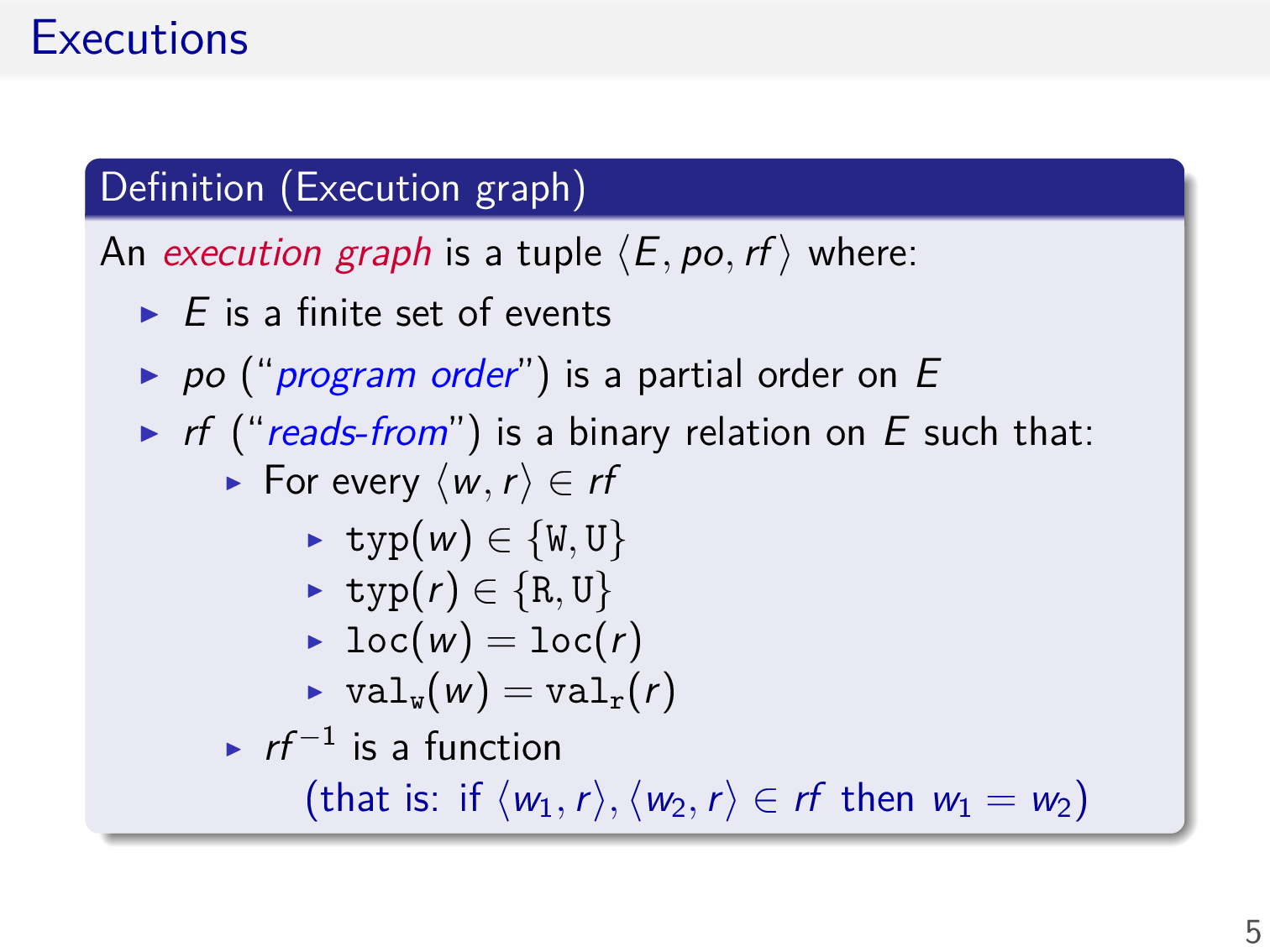
此处形式化定义 Execution graph，顶点就是上述定义的 Events 的有限集，边目前包括下述两种

po，图中顶点的偏序关系，即任意两个顶点之间若存在关系，则必能排出一个序
rf，图中顶点的两元关系，具有如下形式
- 第一个分量的 label 为 $W,U$
- 第二个分量的 label 为 $R,U$
  - 注意到 $U$ 包含了读写两种操作
- 读写的地址是相同的
- 读取的值就是写入的值
- 不存在如下情形

flowchart LR A["W x 0"] --> B["R x"] C["W x 1"] --> B

这里定义了一些记号，主要是为了描述某种类型的顶点或边

Mapping programs to executions

下面需要考虑将程序映射到 execution graph，目前只考虑 po 边

要求该 execution graph 的 po 边为全序关系，即任意两个 events 之间必能排出一个序，这是合理的要求
要求 event 的 tid 为 0，可以参考下面构造该 graph 的流程

这里利用上一节中定义的操作语义，形式化的描述了通过 command 构造 execution graph 的定义

若不访问内存，那么就不存在新的 event，execution graph 不变
若访问内存，选取一个未出现过的 id，置 tid 为 0，加入到 execution graph 中，注意此处 po 的变化，可以保证其为全序关系
- 置 tid 为 0，感觉应该是置 tid 为 thread id

举个例子

x = 1;
y = 1;
a = x; // 1

那么对应的 execution graph 为

flowchart LR A["<0, 0, (W x 1)>"]-->B["<1, 0, (W y 1)>"] B-->C["<2, 0, (R x 1)>"] A-->C

对于给定的 thread，只需选取其中对应的 event，并修改其 tid 为 0，就能得到原图的一个子图

对于一个 graph，若对所有的 thread 执行上述操作，都能得到满足上述定义 (sequential) 的一个子图，则该 graph 即为源程序的一个 execution graph

Consistency predicate

要求 execution graph 满足某些 consistency predicate

例如，要求 rf 边的 codomain 能够取满 read event 的定义域

Sequential consistency

下面使用 declarative semantics 定义 SC

首先 sc 边是 execution graph 的一个全序关系
所有 po 边均为 sc 边
所有 rf 边均为 sc 边，且不存在如下情形

flowchart LR A["<0, 1, (W x 1)>"] --rf--> B["<2, 1, (R x 1)>"] A --sc--> C C["<1, 1, (W x 2)>"] --sc--> B

分析右侧的 execution graph 为何不是 SC

若

flowchart LR A["W x 0"] B["W y 0"] C["W x 1"] D["W y 1"] E["R y 0"] F["R x 0"] A --po--> D B --po--> C A --po--> C B --po--> D C --po--> E D --po--> F A --rf--> F B --rf--> E D --sc--> E

则违反上述定义，又因为 sc 边是全序关系，所以 W y 1 和 R y 0 只能是如下关系，同理可得 W x 1 和 R x 0

flowchart LR A["W x 0"] B["W y 0"] C["W x 1"] D["W y 1"] E["R y 0"] F["R x 0"] A --po--> D B --po--> C A --po--> C B --po--> D C --po--> E D --po--> F A --rf--> F B --rf--> E E --sc--> D F --sc--> C

构造其传递闭包，会发现由于出现了环，违反了全序关系的反对称性，所以不是 SC

还有一种等价的 SC 定义，引入 mo 和 rb 边

注意这里 mo 边实际上构成了对于某个内存地址写的一个全序关系

rb 边定义中的 \id 的含义是去掉 identity 的边，避免 update event 形成自环构成 rb 边

仍然是上述例子，构造其 mo 和 rb 边

flowchart LR A["W x 0"] B["W y 0"] C["W x 1"] D["W y 1"] E["R y 0"] F["R x 0"] A --po--> D B --po--> C A --mo--> C B --mo--> D C --po--> E D --po--> F A --rf--> F B --rf--> E E --rb--> D F --rb--> C

同样形成环

略

Relaxing sequential consistency

略微放松 SC 的语义，即在每个内存地址上实现 SC

这里定义的含义是

⟨a, b⟩ ∈ [RWx]; G.po; [RWx]

顶点 a 和顶点 b 是关于内存地址 x 的读或写的 event，且顶点 a 和 b 之间的边为 po 边

其等价的定义相当于取图中相同内存地址的 po 边，和 rf / mo / rb 边取并集

由于 rf 边和 mo 边的定义保证了其两个顶点一定是对同一个内存地址的 event，所以 rb 边的两个顶点也是对同一个内存地址的 event，这样四者的并集其中的顶点一定是对同一个内存地址的 event

下面人为定义一些 bad patterns，即违反了四者的并集无环的要求

这两个 patterns 很明显

对于 coherence-wr 和 coherence-rr，考虑形成的 rb 边即可

atomicity 同样考虑形成的 rb 边即可

综合上述情形，可以形成对 COH 的另一个等价定义，其证明略

下面来看几个例子

第一个例子，首先画出 po 边和 rf 边

flowchart LR A["W x 0"] B["W x 1"] C["W x 2"] D["R x 2"] E["R x 1"] A --po--> B A --po--> C B --po--> D C --po--> E B --rf--> E C --rf--> D

由于 mo 边为全序关系，所以 W x 1 和 W x 2 之间一定存在一条 mo 边，不妨如下

flowchart LR A["W x 0"] B["W x 1"] C["W x 2"] D["R x 2"] E["R x 1"] A --po--> B A --po--> C B --po--> D C --po--> E B --rf--> E C --rf--> D B --mo--> C E --rb--> C

那么 rb 边和 po 边之间就会形成环，所以在 COH 内存模型下是不被允许的

第二个例子，上面已经分析过了，由于仅考虑每个内存地址上的 SC，所以上述的长度为 4 的环也就不存在了，于是在 COH 内存模型下是被允许的

RA memory model

引子，使用 FAA 指令可以保证在 COH 内存模型下不会出现 a = 1 且 b = 1

考虑使用 CAS 指令实现相同的语义

对于同样的 store buffering 的例子，实际上在 COH 内存模型下，上述情形仍然是被允许的，其根本原因是即使存在 lock，对于一个内存地址的读仍然不能保证其之前的指令对于另一个内存地址的写及时可见

本质上这一种消息传递的编程范式，然而 COH 内存模型并不支持

于是考虑增强 COH 内存模型

即增强 coherence-wr 的能力，从而能够 forbid 更多不合理的情形

例如分析 slide #28 的第二个例子

flowchart LR A["W x 0"] B["W y 0"] C["W x 42"] D["W y 1"] E["R y 1"] F["R x 0"] A --po--> C A --po--> E B --po--> C B --po--> E C --po--> D E --po--> F D --rf--> E A --rf--> F A --mo--> C B --mo--> D F --rb--> C

注意这里 R x 0 -> W x 42 -> W y 1 -> R y 1 构成了环，所以在 RA 内存模型下是不被允许的

需要理解此处的 (po ∪ rf)+ 利用了对另一个内存地址的访问，考虑起点和终点，实际上是 <W x 42, R x 0> ∈ (po ∪ rf)+，仍然是对同一个内存地址的访问，所以没有问题

在 COH 内存模型下，由于缺少了 rf 边，上述闭包就无法构造，于是在 COH 内存模型下是被允许的

这便是 RA 内存模型

存在其等价的定义

第一条等价于 po ∪ rf 无环

略

Towards C/C++11 memory model

考虑弱化 RA 内存模型

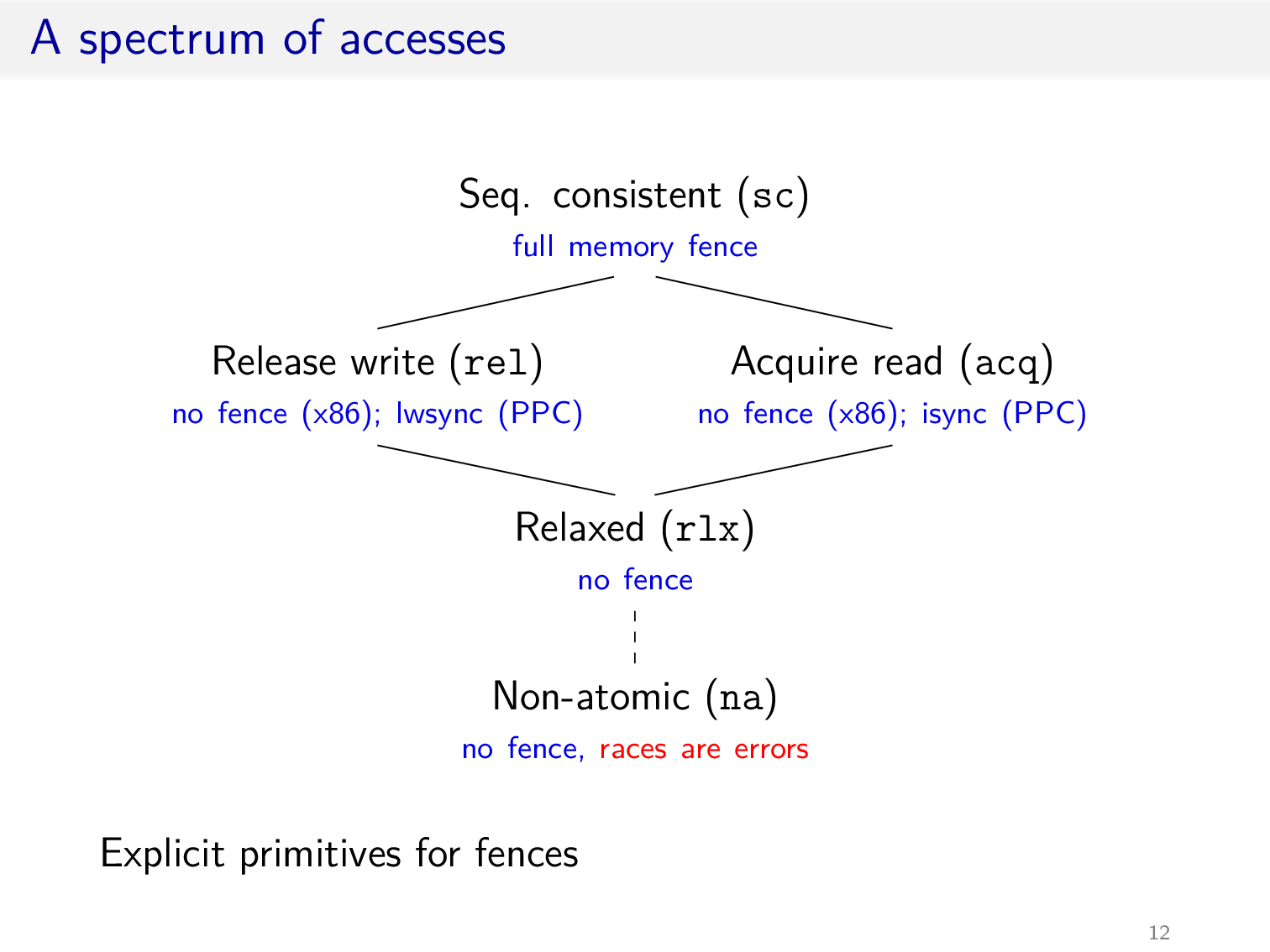
使用 access modes 注解每次内存访问

强于 acq 或 rel 的访问遵循 RA 内存模型，否则遵循 COH 内存模型

由此可以形式化的定义 Happens-Before 的语义，注意这里 synchronizes-with 是一个基本的定义，其中 ⊒ 表示不弱于，下一节会进一步扩充

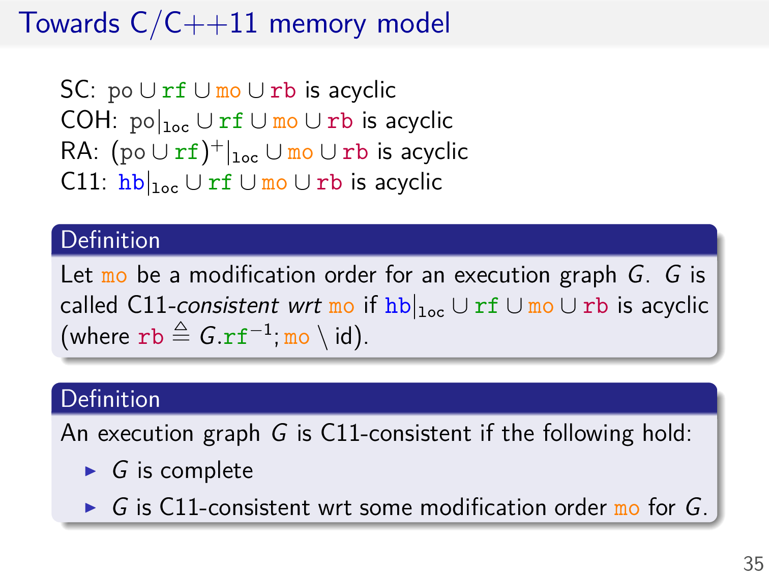
由此可以定义 C11 内存模型

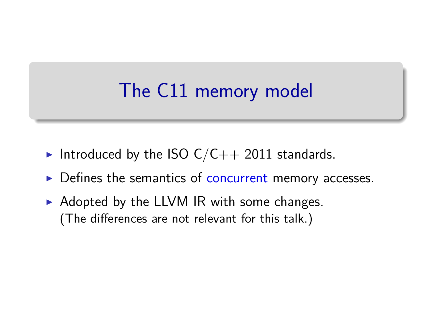
The C/C++11 memory model

较上一节中介绍的 C11 内存模型，这一节会

在存在 data race 的情形下，在 non-atomic 内存模型下程序的行为是未定义的 (catch-fire semantics)
四种类型的 fence
提供 SC 内存模型
更加精细的 synchronizes-with 定义

More elaborate definition of sw

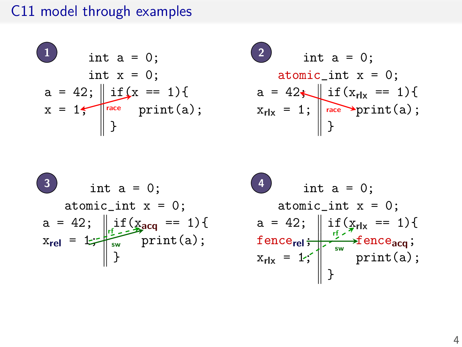
首先是几个例子，对于前两个例子，程序的行为是未定义的，后两个例子则是有定义的

需要在 synchronizes-with 的定义中考虑 fence，加下划线的是添加的部分，本质上就是在 write 前存在 fence，或者在 read 后存在 fence

考虑另外一种情形，此处 FAI 代表 fetch-and-increase，我们希望 rel 和 acq 之间的 update event 不会影响 synchronizes-with 关系的建立

于是只需将 rf 修改为 rf+，由于 rf 边要求是从 write event 指向 read event，所以中间的 event 只可能是 update event

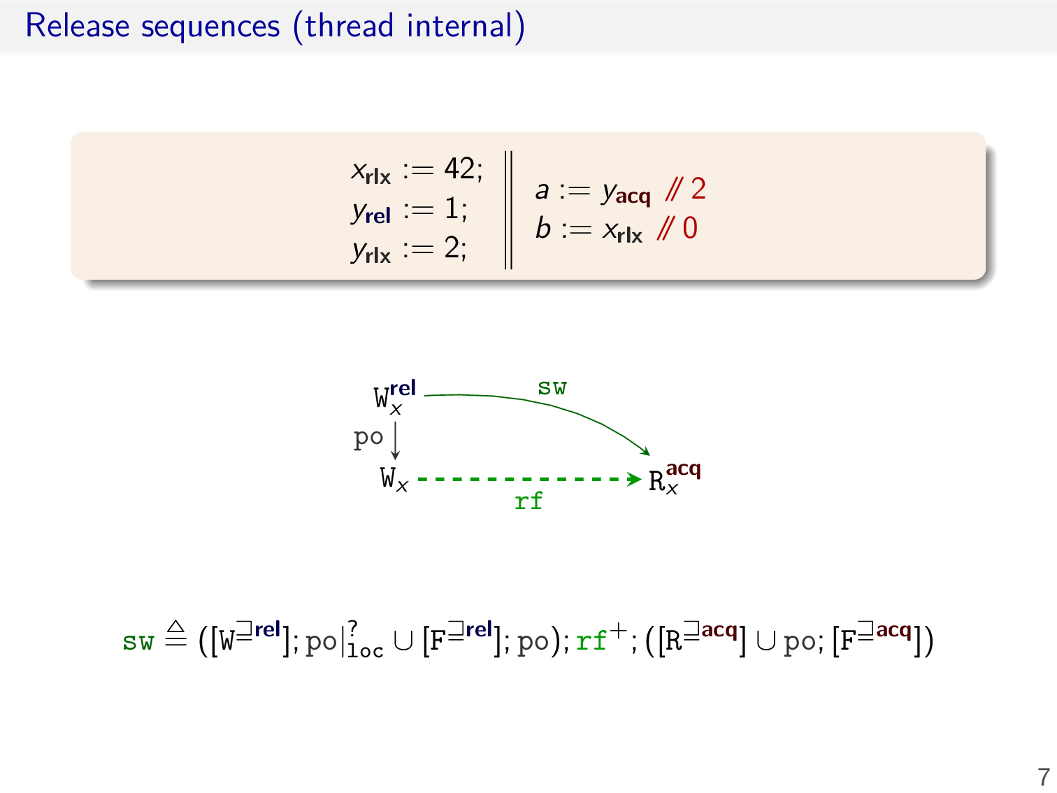
最后一种情形是，我们希望 rel 和 acq 之间对同一个内存地址的任意 access modes 的写不会影响 synchronizes-with 关系的建立，加下划线是修改的部分，其中 ? 代表可有可无

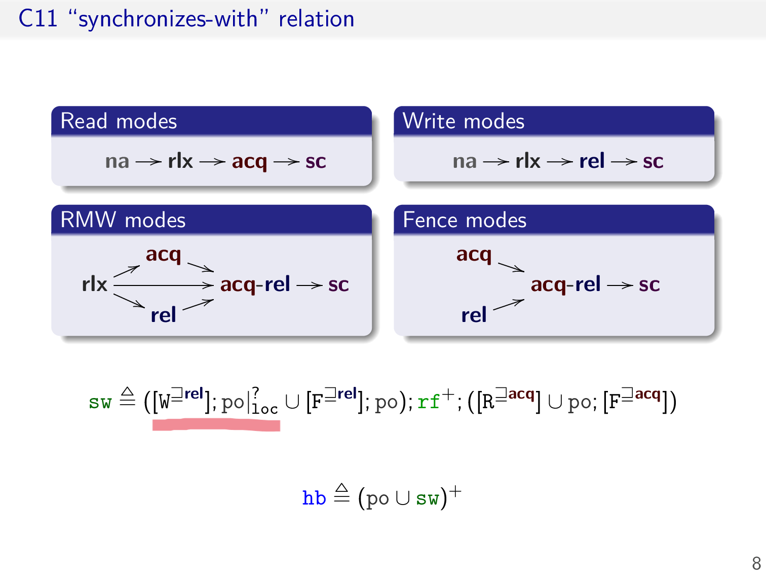
于是在 C11 中，最终的 synchronizes-with 关系定义如上

这里还列举了对 event 所有可能的 access modes，注意这里 na 代表 non-atomic，且 update event 不存在 non-atomic 注解，这与之前操作语义的定义是类似的

Catch-fire semantics

形式化定义何为 data race

对同一个内存地址，至少有一个是写操作
至少有一个操作的 access modes 为 non-atomic
两者之间不存在 Happens-Before 关系

注意这里最后一点可以推导出两个操作一定属于不同的 threads，因为同一个 thread 的 events 之间存在 po 关系

若 execution graph 是 racy 的，那么其 outcome 可以为任意值，即未定义行为

C11 consistency

最后需要考虑在 C11 内存模型中定义 SC 的语义

由于对一个 atomic 变量的访问存在多种 modes (except na)，目前并没有一个完善的定义

对一个普通变量的访问就是 na

上述内容摘自 Repairing sequential consistency in C/C++11

Exercise

为每一次内存访问添加 access modes

这个例子在之前的 Atomic Weapons 中出现过，主要关注 a.count 这个变量

对 a.count 的自增可以是 rlx
对 a.count 的自减需要是 acq-rel，从而保证 free 操作全局即时可见 (消息传递)
- 考虑仅 acq 或仅 rel

TODO

Weak Memory Concurrency in C/C++11 and LLVM

这一节主要批判一下 C11 内存模型，然后引入 promising semantics

Overview

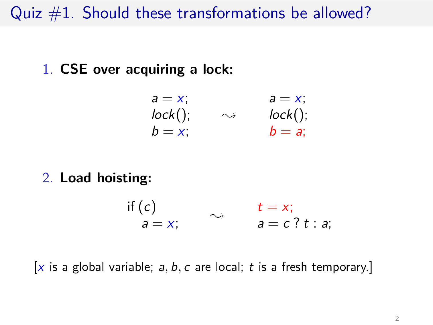
上面是两个常见的编译器优化，其中 hoisting 是利用了 cmov 条件传送指令，以减少分支预测错误的处罚

然而，如果结合上述两种优化，就可能让一个没有 race 的程序产生 race

例如若 c 为 false，那么对 x 的访问就会出现 data race

后面三点在 Memory Models 一节的 Design Criteria 中提过，第一点单调性 (monotone) 在本节 slide #22 会给出解释

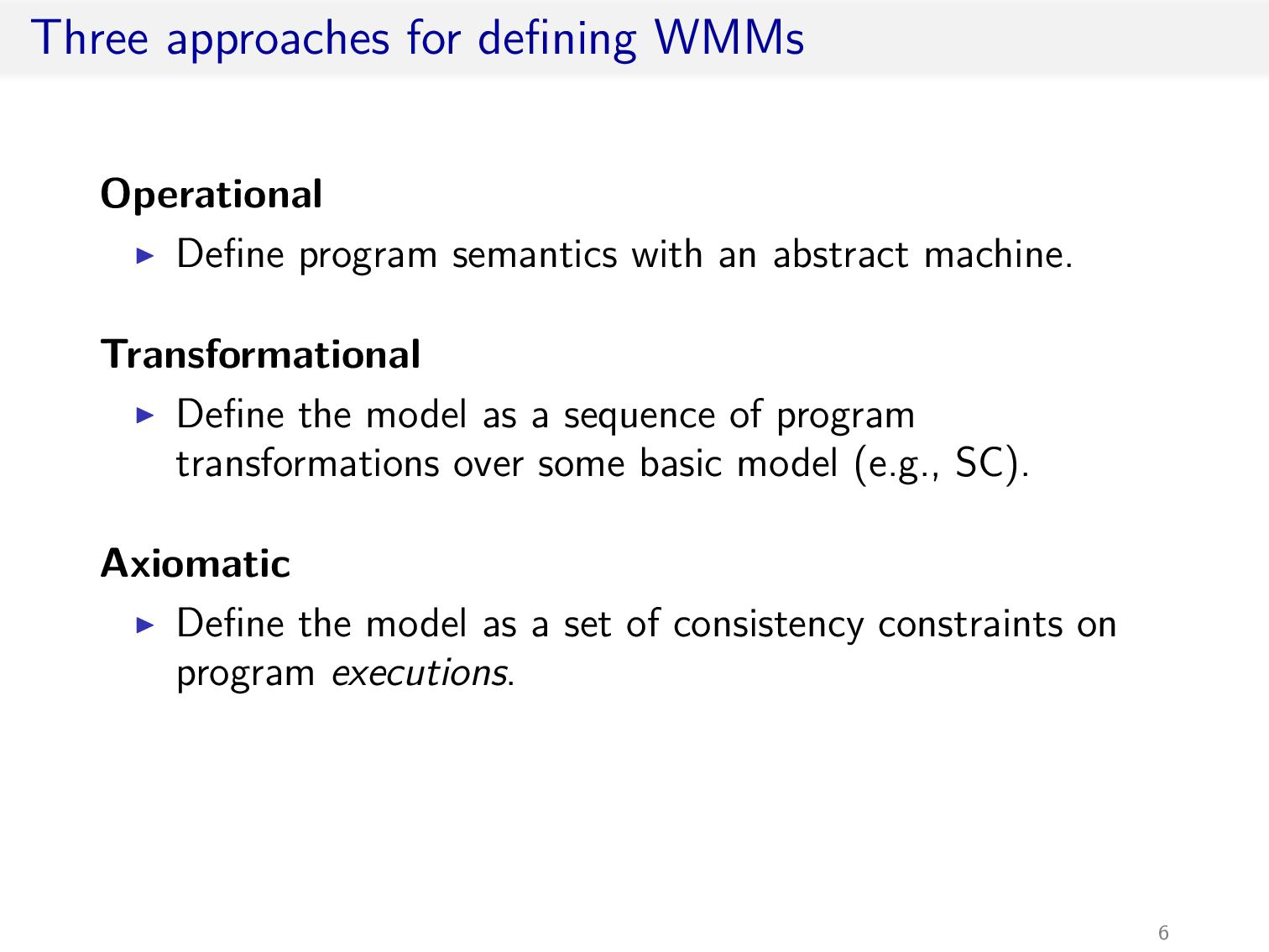
之前讲过了 Operational Semantics 和 Declarative Semantics，后者便是 Axiomatic 的方法，这里略过 Transformational 的方法

The C11 memory model

再次强调，对于 non-atomic 变量，data race 会产生未定义行为，而对于 atomic，就需要考虑可能的 data race 及其合理的行为

注意对变量赋初值是 na access mode，此处 rel 和 acq 形成 sw 边

对于 rlx 版本的 store buffering，C11 内存模型是允许的

对同一个原子变量的 rlx 读写保证不会乱序

Unfortunate flaws in C11

下面是一个例子，说明了 C11 并不保证单调性

在 rlx 读写下，上述构成的 execution graph 无环，所以是被允许的

然而，在 na 读写下，由于 non-atomic read axiom，若发生上述行为，要求 W x 1 和 R x 1 之间要存在 hb 边，然而这是两个不同的 threads，并不存在 hb 边，所以是不可能的

对于 non-atomic read axiom 的说明

<a, b> ∈ rf
mode(b) = na
根据 race 的定义，若不产生 race，必定有 <a, b> ∈ hb 或 <b, a> ∈ hb
若为后者，则 hb ∪ rf 会产生环
所以只可能是 <a, b> ∈ hb

总之 C11 内存模型存在一堆问题

下面还有两个例子

这个例子说明了对于同一个变量不同 access modes 的访问也存在问题

若 R x 0，那么 R x 0 和 W x 1 之间会存在 rb 边，会形成环
若 R x 1，那么 W x 1 和 R x 1 之间应该存在 hb 边，然而这是两个不同的 threads，并不存在 hb 边

所以这里可能读取的值并不合理

这个例子说明了 na read 会阻止一些可能发生的行为

类似上一个例子，若 R a 1，那么 W a 1 和 R a 1 之间应该存在 hb 边，然而这是两个不同的 threads，并不存在 hb 边，所以分支总是为 false，也就破坏了这一节 slide #16 的结构

然而，若串行化前两个线程，由于存在 po 边，W a 1 和 R a 1 之间就存在 hb 边了，程序的行为反而增加了

这实际上就是单调性的丧失，也就是在同步之后程序的行为反而增加了

The OOTA problem

之前提过，在 HMM 内存模型下会出现 OOTA 问题，在 C11 内存模型中同样会出现该问题

C11 内存模型允许 load buffering 行为

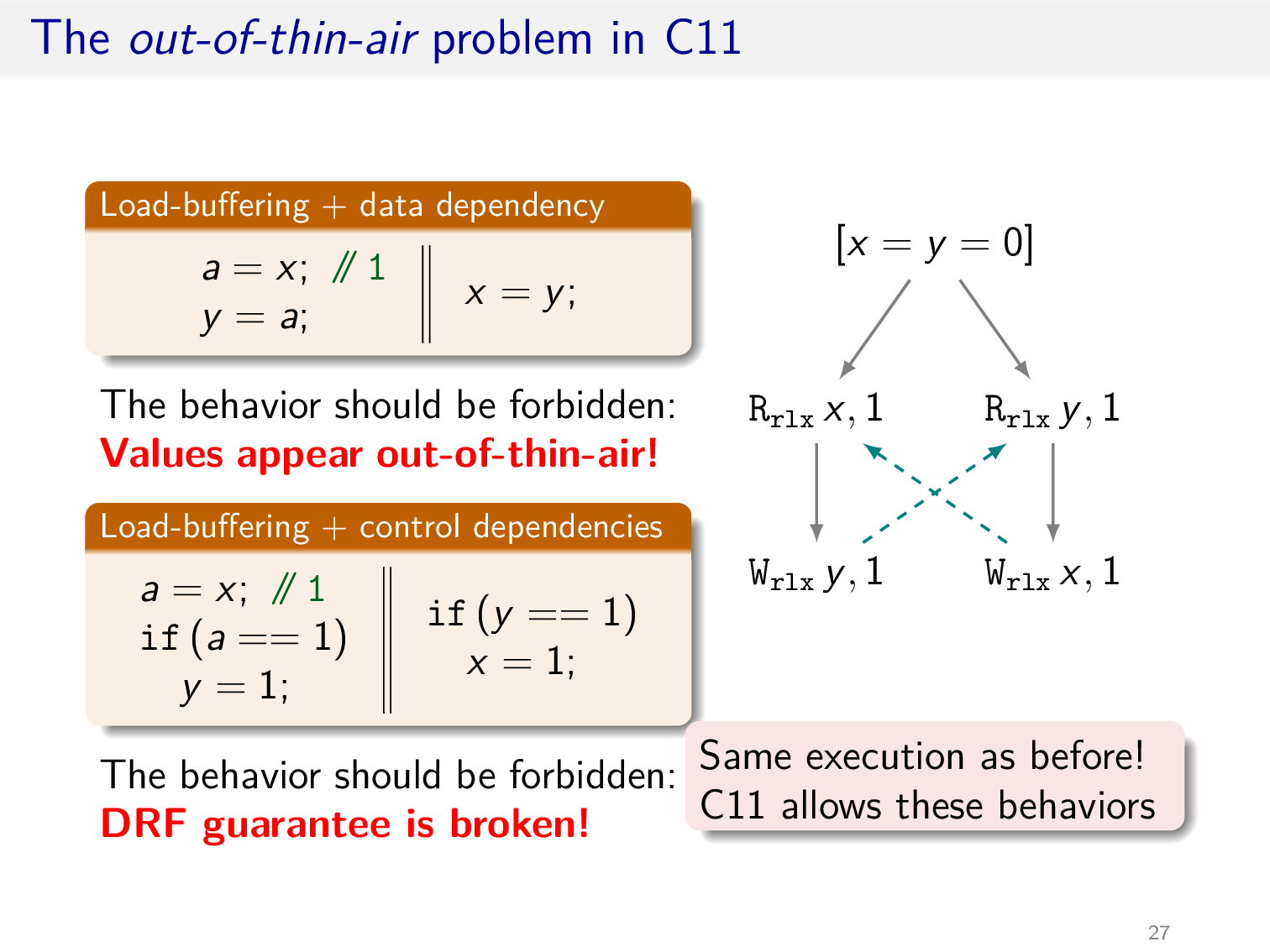
只需略加修改 load buffering，便可以产生 OOTA 问题，此处 a = x 实际上可以读到任意值，然而 execution graph 中并未出现环

另一方面，对于下面的例子，两个线程之间并不存在 race，但却出现了未定义行为，也就违反了 DRF guarantee

在某种程度上，硬件可以解决部分的 OOTA 问题，例如记录数据的依赖关系，加入到 execution graph 中，判断是否存在环，然而会存在误判的情形

A promising solution to OOTA

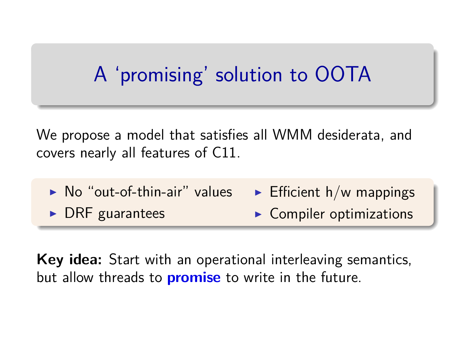
这里通过操作语义提出了一个新的弱内存模型，下面是两个例子

内存现在不是一个 map，而是一些 message 的有序集，对于同一个内存地址而言

每个线程的写操作会向内存中添加 message，其中会额外添加一个 timestamp 实数值，该 timestamp 要大于该线程记录的最大的 timestamp，同时与内存中的所有 timestamps 不同
当一个线程读内存时，可以选择读取 message 集合中大于等于该线程记录的最大的 timestamp 的值，同时更新该线程记录的最大的 timestamp

在 store buffering 的例子中，在 thread #1 的视角下，对 x 的写最新的 timestamp 为 1，而对 y 的写最新的 timestamp 为 0，所以可以读取到 y = 0，thread #2 与之对称

在另一个例子中，在 thread #1 的视角下，对 x 的写最新的 timestamp 为 2，实际上 thread #2 对 x 的写记录的 timestamp 可以在 (0, 1) 之间，此时在 thread #1 的视角下，对 x 的写最新的 timestamp 就变成 1 了

然而，在 thread #2 的视角下，若 thread #1 先写 (timestamp 更小)，那么 thread #2 对 x 的写最新的 timestamp 总是自己记录的 timestamp，所以不可能读到 x 为 1

同理，若 thread #2 先写，那么 thread #1 也不可能读到 x 为 2，所以上述情形不可能发生

下面引入 promise 的概念，一个线程可以将未来的一个写操作添加到内存中，这不会改变该线程记录的最大的 timestamp，但要求在未来的某一时刻，该线程需要完成该写操作，即改变该线程记录的最大的 timestamp

在 load buffering 的例子中，thread #1 在执行前 promise 了 y = 1，添加了 y: 1@1 这个 message，从而 thread #2 能够读取 y 的值，最后，thread #1 更新记录 y 的最大的 timestamp 为 1，所以上述情形是被允许的

这里 promise 能够解决 OOTA 问题关键在于，promise 所承诺的写操作，在线程本地的上下文中，是可以实现的

例如对于最下面的例子，在 thread #1 开始执行前，x 的值为 0，是无法承诺 y = 1 的

下面几个可以加深对 promise 的理解

这里若 promise x = 1，假设 timestamp 为 1，那么在 a = x 读取 x 的值时，就会更新记录 x 的最大的 timestamp 为 1，此时需要 fulfill 之前的 promise，然而之前定义写操作要求该 timestamp 要大于该线程记录的最大的 timestamp，所以这里无法 fulfill，上述行为不被允许

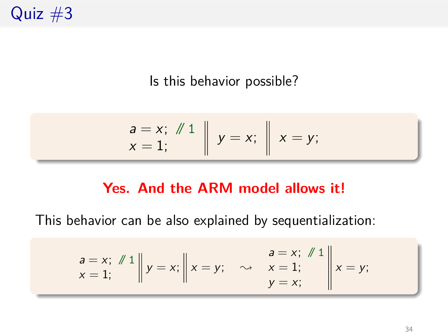
对于上面的例子，若添加两个线程，行为就被允许了，其核心在于在 a = x 读取 x 的值时，所更新的 timestamp 不是之前 promise 的 timestamp，而是 thread #3 进行写操作时设置的 timestamp，若该 timestamp 小于 promise 的 timestamp，x = 1 的 promise 就能成功 fulfill 了

考虑串行化前两个线程，实际上需要 promise x = 1 和 y = 1，由于不会在 thread #1 中读取 y 的值，所以不会影响 y = 1 这个 promise 的 fulfill

然而，这种内存模型下并不是单调的，略加修改上面的例子

先考虑右边，需要 promise y = 1，注意这里 x 的初值为 0，所以分支为 true，promise 在本地上下文中是实现的，在实际的 fulfill 过程中，y 所读取的 x 为 1，实际上发生在 a = x 中，而非分支中

再考虑左边，由于不在一个线程中，无法 promise y = 1，即使 thread #0 promise x = 1，由于 a 最终的值为 1，所以分支为 false，无法执行到写操作对应的指令

目前只考虑了 na access，完整的内存模型还需要考虑很多东西

以 rel 和 acq access modes 为例，当一个写操作为 rel 时，需要在 message 中添加当前线程的 view，这样另一个线程 acq 对应的写操作时，可以应用其余变量的 timestamp，进而实现同步

Concurrent Objects

Safety and Liveness

Safety (Correctness)

those properties whose violation always has a finite witness

if something bad happens on an infinite run, then it happens already on some finite prefix

Liveness (Progress)

those properties whose violation never has a finite witness

no matter what happens along a finite run, something good could still happen later

Correctness

Sequential Specifications

If (precondition)
- the object is in such-and-such a state before you call the method,
Then (postcondition)
- the method will return a particular value or throw a particular exception,
and (postcondition, con’t)
- the object will be in some other state when the method returns.

Example: Pre and PostConditions for Dequeue

Precondition:

Queue is non-empty

Postcondition:

Returns first item in queue

Postcondition:

Removes first item in queue

Precondition:

Queue is empty

Postcondition:

Throws Empty exception

Postcondition:

Queue state unchanged

Sequential vs. Concurrent

Sequential:
- Object needs meaningful state only between method calls
Concurrent:
- Because method calls overlap, object might never be between method calls

Sequential:
- Each method described in isolation
Concurrent:
- Must characterize all possible interactions with concurrent calls

Sequential:
- Can add new methods without affecting older methods
Concurrent:
- Everything can potentially interact with everything else

Linearizability intuition

Each method should
- take effect
- Instantaneously
- Between invocation and response events
Sounds like a property of an execution
A linearizable object: one all of whose possible executions are linearizable

Formal Model of Executions

Invocation Notation

A q.enq(x)

Response Notation

A q:void

History

Describing an Execution

H

A q.enq(3)
A q:void
A q.enq(5)
B p.enq(4)
B p:void
B q.deq()
B q:3

Match

Invocation & response match if

Thread names agree
Object names agree

Projections

Object Projections

H|q

A q.enq(3)
A q:void
A q.enq(5)
B q.deq()
B q:3

Thread Projections

H|A

A q.enq(3)
A q:void
A q.enq(5)

Complete Subhistory

An invocation is pending if it has no matching respnse

no unmatched Invocation & response

Complete(H)

A q.enq(3)
A q:void
B p.enq(4)
B p:void
B q.deq()
B q:3

Sequential Histories

Method calls do not interleave

Well-Formed Histories

Per-thread projections sequential, avoid

A q.enq(3)
A q.enq(4)

Equivalent Histories

Threads see the same thing in both, ∀A. H|A = G|A

Sequential Specifications

A sequential specification is some way of telling whether a single-thread, single-object history is legal
A sequential (multi-object) history H is legal if for every object x, H|x is in the sequential spec for x

Precedence

A method call precedes another if response event precedes invocation event

Given history H, method executions m0 and m1 in H, We say m0 ->H m1, if m0 precedes m1

Relation ->H is a partial order, total order if H is sequential

Linearizability

History H is linearizable if it can be extended to G by

Appending zero or more responses to pending invocations
Discarding other pending invocations

So that G is equivalent to legal sequential history S, where ->G ⊆ ->S

legal defined by sequential specification

S respects “real-time order” of G

Composability Theorem

History H is linearizable if and only if, for every object x, H|x is linearizable

Linearization point

Identify one atomic step where method happens

Might need to define several different steps for a given method

Example:

public T deq() throws EmptyException {
  lock.lock();
  try {
    if (tail == head)
       throw new EmptyException();
    T x = items[head % items.length];
    head++;
    return x;
  } finally {
    lock.unlock();
  }
}

the moment of unlock

Sequential Consistency

History H is sequential consistency if it can be extended to G by

Appending zero or more responses to pending invocations
Discarding other pending invocations

So that G is equivalent to legal sequential history S

No ->G ⊆ ->S

No need to preserve real-time order

Often used to describe multiprocessor memory architectures

Sequential Consistency does not have composability

视整个 memory 为一个 object，若该 object 满足 sequential consistency，则该 memory model 是 SC 的

Example:

实际上是 store buffering

Initially:  x = y = 0

// thread 1
x = 1;
r1 = y; // 0

// thread 2
y = 1;
r2 = x; // 0

H|x 和 H|y 都是 SC 的，但是 H 是 TSO，是弱于 SC 的

Progress

Progress Conditions

Deadlock-free: some thread trying to acquire the lock eventually succeeds.
Starvation-free: every thread trying to acquire the lock eventually succeeds.
Lock-free: some thread calling a method eventually returns.
Wait-free: every thread calling a method eventually returns.

	Non-Blocking	Blocking
Everyone makes progress	Wait-free	Starvation-free
Someone makes progress	Lock-free	Deadlock-free

blocking progress conditions depend on fair scheduler

Summary

We will look at linearizable blocking and non-blocking implementations of objects.

Linked lists

Target

adding threads should not lower throughput
- e.g. CAS invalidate cache line
should increase throughput

Four Patterns

Fine-Grained Synchronization
Optimistic Synchronization
Lazy Synchronization
Lock-Free Synchronization

Set Interface

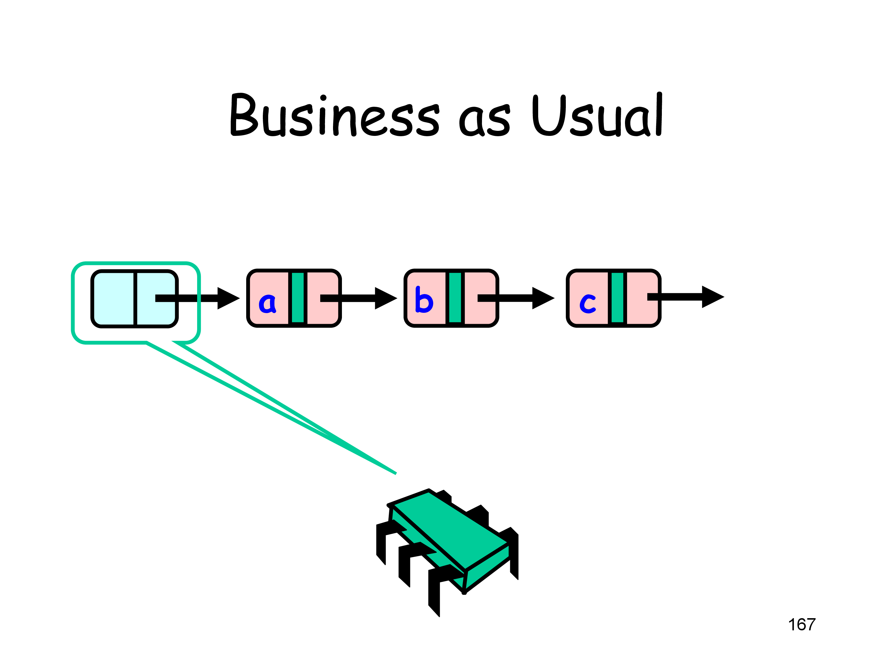
public interface Set<T> {
    public boolean add(T x);
    public boolean remove(T x);
    public boolean contains(T x);
}

List Node

public class Node {
    public T item;
    public int key;
    public Node next;
}

Representation Invariant

Sentinel nodes
- tail reachable from head
Sorted (by key)
No duplicates

Abstraction Map

Given a list satisfying rep invariant, S(head) = { x | there exists a such that a reachable from head and a.item = x}

Fine-Grained Synchronization

由于 Coarse-Grained Locking 的策略，即一把大锁保平安，lock 的 contention 过于严重

考虑将 lock 拆分，即 Fine-Grained Synchronization

基本思想是持有两把 locks，通过交替 lock 和 unlock，在 list 中搜索然后完成相应的操作

下面是一个并发 remove 的例子

Linearization point 只需选取持有对应的 locks 之后实际对 list 进行操作的任意时刻即可

Progress 的性质取决于 head 节点上 lock 的性质

Optimistic Synchronization

基本思想

Find nodes without locking
Lock nodes
Check that everything is OK (validate)

validate 需要考虑下面两点

给定的节点是否仍然可达
prev 是否依然指向 cur

Lazy Synchronization

Like optimistic, except

scan once
contains(x) never locks

主要思想是为每一个节点添加一个 field，用于表示该节点是否被 marked delete，在做实际的 delete 操作前，设置该 field，在 SC 内存模型下，其余线程就可以得知自己 scan 到的节点是否仍然存在，从而避免了 rescan

validate 需要考虑下面两点

prev 和 cur 是否被 marked delete
prev 是否依然指向 cur

还需要更新 Abstraction Map 的定义

Given a list satisfying rep invariant, S(head) = { x | there exists a such that a reachable from head, a.item = x and a is unmarked}

注意到此时的 contains 操作实际上是 wait-free 的

Lock-Free Synchronization

避免使用 lock，考虑使用 CAS 操作

例如删除 cur 所在的节点，只需如下操作

prev.next.CAS(cur, succ);

然而存在一种情形，即 prev 已经被 marked delete，此处上述操作就会出现问题

于是在进行 CAS 操作的时候需要同时考虑 mark 字段

JAVA 提供了 AtomicMarkableReference 类

这样，在删除 cur 所在的节点时，需要如下操作

if (!prev.next.attemptMark(cur, true)) {
    continue;
}
Node<T> succ = cur.next.getReference();
prev.next.compareAndSet(cur, succ, true, false);
return true;

logical remove，置 prev.next 的 mark 为 true
- 若该操作失败，代表 list 的结构已发生变化，需要重新 scan
physical remove，若 prev.next == cur 且 prev.next 的 flag 为 true，则置 prev.next = succ，且 prev.next 的 flag 为 false
- 若该操作失败，代表其余线程在 scan 的过程中，已经 physical remove 了 cur 所在的节点，于是直接返回即可

这里的想法是，每个线程在 scan 的过程会 active 的 physical remove 已经被 logical remove 的节点，避免因为一个线程因为某些原因始终无法 physical remove 对应的节点，进而形成类似 lock 的效应

对于 add 方法，当 physical add 操作失败，代表 list 的结构已发生变化，需要重新 scan

于是，在 contains 操作是 wait-free 的基础上，add 和 remove 操作变成了 lock-free

在性能方面，Lock-Free Synchronization 相较于 Lazy Synchronization 提升并不明显，因为算法更加复杂了

Queues

Bounded, Blocking, Lock-based Queue

这里 blocking 的含义是

若 queue 为 full，对 queue 执行 enq 操作会阻塞，直到其他线程执行了 deq 操作
若 queue 为 empty，对 queue 执行 deq 操作会阻塞，直到其他线程执行了 enq 操作

很显然，线程之间消息的传递需要使用条件变量

由于 enq 操作和 deq 操作分别在 queue 的两端进行，所以需要两把 locks，每把 lock 对应一个条件变量

以 enq 操作为例，deq 操作与其完全对称

首先获取 enq lock
判断 queue 的大小是否超过容量，若是，则 wait
否则在 tail 侧执行实际的 enq 操作，这也是对应的 linearization point
自增 queue 的大小，并释放 enq lock
若此前 queue 为 empty，需要唤醒所有的 deq 线程
- 使用 signalAll 而非使用 signal，是为了避免 Lost Wake-Up 问题
- 关于 Java 的 concurrent primitives，在此不深究

简单起见，这里 queue 的大小使用一个原子变量记录，自增和自减该原子变量会在 enq 线程和 deq 线程之间形成 contention

一种解决方案是，enq 操作和 deq 操作分别维护一个变量 queue 的大小，当变量 overflow 或 underflow 时，同时获取 enq lock 和 deq lock，以此同步 queue 的真实大小

Unbounded, Non-Blocking, Lock-free Queue

这里 non-blocking 在 unbounded 语境下的含义是

若 queue 为 empty，对 queue 执行 deq 操作会抛出 exception

考虑使用 CAS 操作修改 queue，以 enq 为例，需要修改两处地方

tail.next = node
tail = node

显然一次 CAS 操作只能修改一个地方，若两次 CAS 操作之间被其他线程打断，queue 就会陷入异常的状态

这里的想法和 Lock-Free 类似，即

视第一次操作为 logical enq，若失败，则重试
对于第二次操作，实际上其 precondition 为 tail.next != null，无论是 enq 线程还是 deq 线程，只要发现上述 precondition 成立，均可以进行第二次操作
- 也就是说，对于 enq 而言，即使对应的第二次操作失败，也可以直接返回

enq 操作的核心代码可以参考

while (true) {
    Node<T> last = tail.get();
    Node<T> next = last.next.get();

    // optimize
    if (last != tail.get()) {
        continue;
    }

    if (next == null) {
        if (last.next.compareAndSet(null, node)) {
            tail.compareAndSet(last, node);
            return;
        }
    } else {
        // help
        tail.compareAndSet(last, next);
    }
}

当 logical enq 成功之后，即第 11 行的分支为 true，此后到 return 之间的任意时刻均可作为 linearization point

deq 操作的核心代码可以参考

while (true) {
    Node<T> first = head.get(), last = tail.get();
    Node<T> next = first.next.get(); // <--

    // optimize
    if (first != head.get()) {
        continue;
    }

    if (first == last) {
        if (next == null) {
            // empty
            throw new EmptyException();
        }
        // help
        tail.compareAndSet(last, next);
    } else if (head.compareAndSet(first, next)) {
        return next.item;
    }
}

这里比较 tricky 的地方在于，对于 throw exception 情形下 linearization point 的选择

若选择第 11 行的分支为 true 之后的某一时刻作为 linearization point，由于可能在该分支之后其余线程执行了 enq 操作，所以并不合理

实际上应当选取第 3 行原子的读取到 next 为 null 的时刻作为 linearization point，同时保证在这一轮能够执行到 throw exception 那一行，即该 linearization point 是 future-dependent 的

The Dreaded ABA Problem

在上述 Lock-free Queue 的流程中考虑手动管理内存

一个简单的想法是，在全局维护一个 free list，其中存放了 unused queue nodes

进行 enq 操作时，向 list 中 pop node
进行 deq 操作时，向 list 中 push node

由于 CAS 操作只会比较 node 的地址，而不会比较该地址中存放的内容，所以可能出现 Dreaded ABA Problem

这里的流程是，一个线程想要进行 deq 操作，然后该线程睡眠，期间有另一个线程进行了一些 deq 和 enq 操作，导致原来 head 指针指向的 node 被回收，然后又被 reuse 成为 head 指针指向的 node，此时该 node 其中的内容已经发生了改变，但是由于该 node 的地址没有发生变化，所以刚开始的线程进行的 CAS 操作仍然会成功，从而使 queue 陷入异常的状态

出现 Dreaded ABA Problem 的根本原因是 CAS 指令的语义，如果使用 Load-link/store-conditional 指令，在 store 的时候会检查从 load 到 store 这段时间内，该地址存放的内容是否发生了变化，使用 LL/SC 代替 CAS 实现上述 Lock-free Queue，就不会出现 Dreaded ABA Problem

如果只能使用 CAS 操作，类似 Lock-Free List 中的想法，在进行 CAS 操作的时候考虑对应的 stamp 字段，该字段记录了该地址存放的内容被修改的时间

JAVA 提供了 AtomicStampedReference 类

Stacks

Lock-free Stack

类似 Lock-free Queue，不过由于 push 和 pop 仅需一次 CAS 操作，所以实现会简单很多

对比 enq 和 push，enq 需要设置 tail.next 和 tail，而 push 仅需要设置 top，对于 node.next = top 的设置并不会修改 stack 本身

若 push 或 pop 失败，该线程会随机的 sleep 一段时间 (backoff)，然后重试该请求

Lock-free Stack 不是 wait-free 的，可能存在某个调度序列，导致某个请求始终无法返回

Linearization point 只需选取对 stack 实际进行修改的时刻即可

Lock-free Stack 一些缺陷

Without GC, fear ABA
Without backoff, huge contention at top

Elimination-backoff Stack

考虑上述 Lock-free Stack 的第二点缺陷，当 CAS 操作失败时，线程会随机的 sleep 一段时间，然后重试该请求，为了避免 contention，随着重试次数增加，sleep 的时间也可以相应增加

观察到一种现象，即存在两个线程配对的 push 和 pop，由于 CAS 操作失败，两个线程都会 sleep

实际上可以考虑让 push 的线程将 value 存放在一个 array 随机的一个位置，然后等待 pop 的线程用 null value 与该 value 交换，从而实现 stack 的语义

对称的，pop 的线程将 null value 存放在一个 array 随机的一个位置，然后等待 push 的线程用 value 与该 null value 交换，同样可以实现 stack 的语义

更具体的

push 和 pop 操作仍然首先通过 CAS 操作与 top 交互
当 CAS 操作失败，则考虑通过一个 elimination array，试图交换 push 的 value 和 pop 的 null value
若交换失败，继续通过 CAS 操作与 top 交互，即重复上述操作

这样可以优化 backoff 的纯 sleep 带来的并发度的下降

对于具体的交换操作，有一些参数可以设置

elimination array 的大小，可以随着 CAS 操作失败的频率动态变化，也可以通过调整 push 和 pop 能够访问该 array 的 range 来实现
push 和 pop 的线程等待交换的时间，随着重试次数增加，等待交换的时间也可以相应增加

上述算法的核心在于 elimination array 中一个 slot 的实现，考虑使用无锁的方式实现，称之为 Lock Free Exchanger

每个 slot 存在着如下状态

empty - nothing yet
waiting - one thread is waiting for rendez-vous
busy - other threads busywith rendez-vous

由于状态数超过了 2，具体实现可以考虑使用 AtomicStampedReference

状态间的转移如下，细节详见代码注释

T item = slot.get(stamp); // 首先读取状态
switch (stamp[0]) {
case EMPTY: {
    if (!slot.compareAndSet(item, myItem, EMPTY, WAITING)) { // 若 CAS 操作失败，代表该 slot 已经被其余线程修改，重试
        break;
    }

    while (System.currentTimeMillis() < timeBound) { // 在时限内不断检测是否有另一个线程交换了 value
        item = slot.get(stamp);
        if (stamp[0] == BUSY) { // 若有，则重置状态，并返回交换的 value
            slot.set(null, EMPTY);
            return item;
        }
    }

    if (slot.compareAndSet(item, null, WAITING, EMPTY)) { // 超时，试图重置状态
        throw new TimeoutException();
    }

    item = slot.get(stamp); // 重置失败，代表在超时后有另一个线程交换了 value，于是重置状态，并返回交换的 value
    slot.set(null, EMPTY);
    return item;
}
case WAITING: {
    if (slot.compareAndSet(item, myItem, WAITING, BUSY)) { // 该 slot 中存在 value 正在等待被交换，尝试进行交换操作
        return item;
    }
    break;
}
case BUSY: { // 有两个线程正在使用该 slot 进行交换，直接返回
    break;
}
default:
    assert false;
}

对于 Safety 和 Liveness 的分析如下

linearizable
- 显然与 stack 的直接交互是 linearizable 的
- 与 elimination array 的交互，只需选取上述 return item 的时刻作为 linearization point 即可
- 考虑到 linearizable 的 composability theorem，所以是 linearizable 的
lock free
- 仍然可能存在某个调度序列，导致某个请求始终无法返回

The Relative Power of Synchronization Operations

The Art of Multiprocessor Programming Chapter 5

在 wait free 的基础上，考虑各种 current objects 能够实现几个线程之间的 consensus

简单起见，这里的 consensus 所 decide 的 value 定义为第一个 propose 的线程所提供的 value

注解

Lock-Free vs. Wait-free

Any wait-free implementation is lock-free.

Lock-free is the same as wait-free if the execution is finite.

下述的一系列结论在 lock free 的基础上也成立

Consensus is universal

See Chapter 6

Consensus Numbers

一个 current object 对应的 consensus number n 定义如下

if it can be used to solve n-thread consensus, take any number of instances of X together with atomic read-write registers and implement n-thread consensus
but not (n+1)-thread consensus

可以证明 atomic read-write registers 的 consensus number 为 1

FIFO Queue

我们想要了解能否只使用 atomic read-write registers 实现一个 FIFO Queue (multiple dequeuers or multiple enqueuers)

single-enqueuer and single-dequeuer 的 Queue 可以通过 atomic read-write registers 实现

    public class WaitFreeQueue {
        int head = 0, tail = 0;
        Item[size] items;

        public void enq(Item x) {
            while (tail - head == QSIZE) {}
            items[tail % QSIZE] = x;
            tail++;
        }

        public Item deq() {
            while (tail - head == 0) {}
            Item item = items[head % QSIZE];
            head++;
            return item;
        }
    }

考虑使用反证法，如果能够通过 FIFO Queue 实现 2-thread consensus，那么 atomic read-write registers 的 consensus number 就为 2，矛盾

所以需要考虑如何通过 FIFO Queue 实现 2-thread consensus

其构造并不困难，两个线程并发的对 FIFO Queue 执行 deq 操作，所 decide 的 value 定义为取到 FIFO Queue 的第一个元素的线程所提供的 value 即可

这也代表 FIFO Queue 的 consensus number 至少为 2

Multiple Assignment Theorem

Atomic registers cannot implement multiple assignment

其证明思路也是反证法，take 3-element array

A writes atomically to slots 0 and 1
B writes atomically to slots 1 and 2
Any thread can scan any set of locations

可以证明 double assignment 的 consensus number 至少为 2

Read-Modify-Write

考虑在硬件层面提供一种特殊的寄存器，该寄存器支持 RMW 操作，可以抽象为

public abstract class RMWRegister {
    private int value;

    synchronized public int getAndMumble() {
        int prior = this.value;
        this.value = mumble(this.value);
        return prior;
    }
}

其中的 mumble 是一个 function

对于普通的 read，mumble 即为 $\lambda x.x$
对于 FAA，mumble 即为 $\lambda x.x + a$
对于 CAS，mumble 会更加复杂

下面给出 non-trivial 的定义

A RMW method with function mumble(x) is non-trivial if there exists a value v such that v ≠ mumble(v)

显然对于普通的 read，其对应的 RMW object 是 trivial 的

可以证明 non-trivial RMW object 的 consensus number 至少为 2

public class RMWConsensus
        extends ConsensusProtocol {
    private RMWRegister r = v;

    public Object decide(object value) {
        propose(value);
        if (r.getAndMumble() == v)
            return proposed[i];
        else
            return proposed[j];
    }
}

其中的初值 v 要求 v ≠ mumble(v)

有一类特殊的 RMW objects，其 mumble functions 属于 $\mathcal{F}$

Let $\mathcal{F}$ be a set of functions such that for all $f_i$ and $f_j$ , either

Commute: $\forall v.f_i(f_j(v))=f_j(f_i(v))$

Overwrite: $\forall v.f_i(f_j(v))=f_i(v)$

可以证明它们的 consensus number 为 2

对于 FAA，其 mumble function 满足 Commute 性质，所以其对应的 RMW object 的 consensus number 为 2

对于 CAS，可以证明其对应的 RMW object 的 consensus number 为 $\infty$

public class RMWConsensus
        extends ConsensusProtocol {
    private AtomicInteger r =
            new AtomicInteger(-1);

    public Object decide(object value) {
        propose(value);
        r.compareAndSet(-1, i);
        return proposed[r.get()];
    }
}

这里 i 代表线程编号，所以选取 -1 为初值

并发算法与理论

TOC

Info

Overview

Concurrent Program

Memory Models

Course Overview

Memory Models

Design Criteria

Happens-Before Memory Model (HMM)

good speculation

bad speculation

JMM

Operational Semantics

Basic domains

Expressions and commands

Programs

The thread subsystem

Store

State

Transitions

SC storage subsystem

Machine state

Transitions

Lifting to concurrent programs

State

Transition

Linking the thread and storage subsystems

Transition

Allowed outcome

TSO storage subsystem

PSO storage subsystem

Declarative Semantics

Executions

Mapping programs to executions

Consistency predicate

Sequential consistency

Relaxing sequential consistency

RA memory model

Towards C/C++11 memory model

The C/C++11 memory model

More elaborate definition of sw

Catch-fire semantics

C11 consistency

Exercise

Weak Memory Concurrency in C/C++11 and LLVM

Overview

The C11 memory model

Unfortunate flaws in C11

The OOTA problem

A promising solution to OOTA

Concurrent Objects

Safety and Liveness

Safety (Correctness)

Liveness (Progress)

Correctness

Sequential Specifications

Sequential vs. Concurrent

Linearizability intuition

Formal Model of Executions

Invocation Notation

Response Notation

History

Match

Projections

Complete Subhistory

Sequential Histories

Well-Formed Histories

Equivalent Histories

Sequential Specifications

Precedence

Linearizability

Composability Theorem

Linearization point

Sequential Consistency

Progress

Progress Conditions

Summary

Linked lists

Target