TOC
Open TOC
- info
- hw ref
- compiler
- mugrade
- 1 - Introduction / Logistics
- 2 - ML Refresher / Softmax Regression
- 3 - Manual Neural Networks / Backprop
- hw0
- 4 - Automatic Differentiation
- 5 - Automatic Differentiation Implementation
- hw1
- 6 - Optimization
- 7 - Neural Network Library Abstractions
- 8 - NN Library Implementation
- 9 - Initialization, Normalization and Regularization
- hw2
- 11 - Hardware Acceleration
- 12 - GPU Acceleration
- 13 - Hardware Acceleration Implementation
- hw3
- 10 - Convolutional Networks
- 14 - Convoluations Network Implementation
info
hw ref
https://github.com/zeyuanyin/hw1
https://github.com/zeyuanyin/hw2
https://github.com/wzbitl/needle
compiler
mugrade
https://mugrade-online.dlsyscourse.org/
- email: 201250012@smail.nju.edu.cn
- token:
xxx
其测试用例在本地运行,并将结果发送到 mugrade 中进行比对
1 - Introduction / Logistics
Why study deep learning systems?
- To build deep learning systems.
- To use existing systems more effectively.
- Deep learning systems are fun!
Elements of deep learning systems
- Compose multiple tensor operations to build modern machine learning models
- Transform a sequence of operations (automatic differentiation)
- Accelerate computation via specialized hardware
- Extend more hardware backends, more operators
2 - ML Refresher / Softmax Regression
Three ingredients of a machine learning algorithm
- The hypothesis class: the “program structure”, parameterized via a set of parameters, that describes how we map inputs (e.g., images of digits) to outputs (e.g., class labels, or probabilities of different class labels)
- The loss function: a function that specifies how “well” a given hypothesis (i.e., a choice of parameters) performs on the task of interest
- An optimization method: a procedure for determining a set of parameters that (approximately) minimize the sum of losses over the training set
Softmax Regression
Setting
k-class classification,多分类问题
Training data:
- = dimensionality of the input data
- = number of different classes / labels
- = number of points in the training set
The hypothesis class
刻画了对于输入数据 ,其标签为 的可能性,可以认为输出为
这里考虑 linear hypothesis function
若记 ,则有 batch 形式
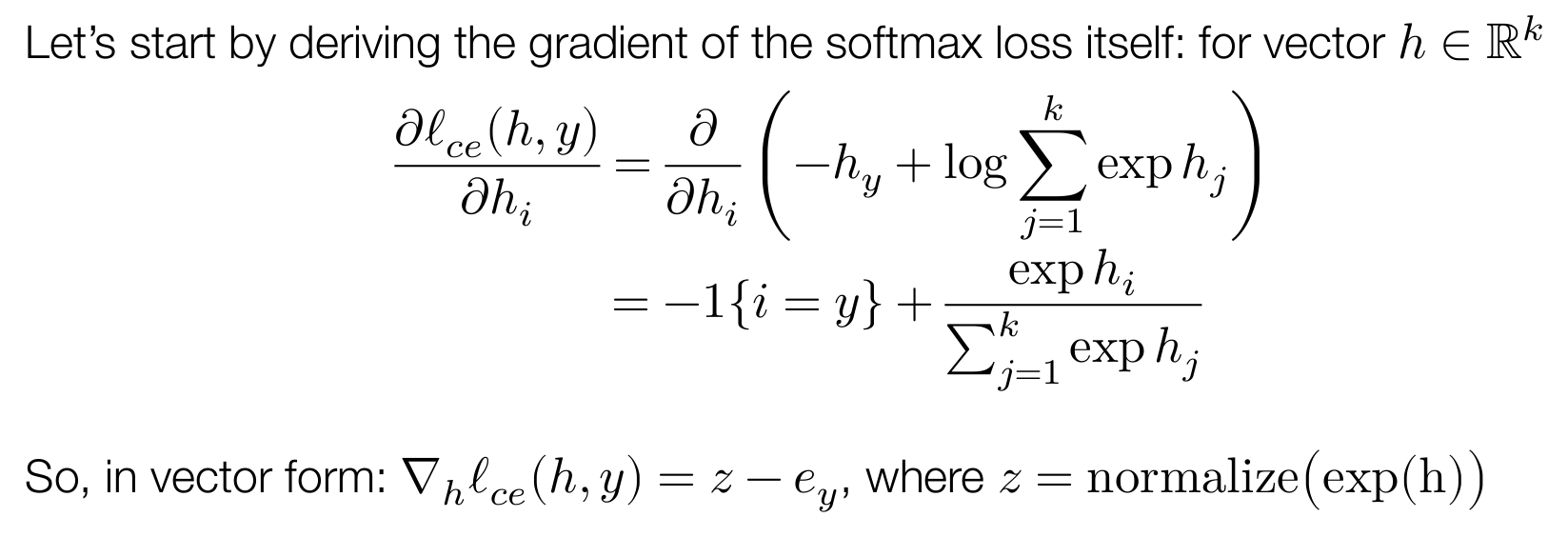
The loss function
softmax / cross-entropy loss
定义
那么
An optimization method
对于 linear softmax regression,我们的目标是
考虑使用 stochastic gradient descent (SGD),即选取输入数据一个大小为 的 minibatch,使用如下方式更新参数
其中 为学习率,转换为 batch 形式
可以证明
其中
且 ,其构造如下
y_identity = np.zeros((batch, num_classes))for j in range(batch): y_identity[j][y_batch[j]] = 13 - Manual Neural Networks / Backprop
From linear to nonlinear hypothesis classes
考虑非线性的 hypothesis function
这里的 可以为非线性函数,更具体的,定义
一般而言 会预先设定好,此时 中的 代表了
Neural networks
A neural network refers to a particular type of hypothesis class, consisting of multiple, parameterized differentiable functions (a.k.a. “layers”) composed together in any manner to form the output.
”Deep network” is just a synonym for “neural network,” and “deep learning” just means “machine learning using a neural network hypothesis class”.
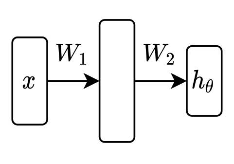
Two layer
batch 形式如下
Universal function approximation
略去,此处大概说明了二层的神经网络可以拟合任意连续的非线性函数
高拟合的代价,参数膨胀
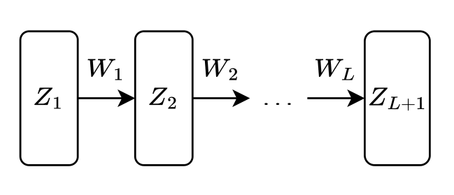
L layer
注意当取 为 时,其形式与上述 Two layer 的神经网络有略微不同
取 即可
为简单起见,省略偏置部分,如
这里直接给出了 batch 形式,原始形式如下
稍微解读一下 batch 形式,实际上
将 个 组合成 的矩阵
而
将 广播为
实际上完整的操作如下
Backpropagation
考虑对 Two layer 的神经网络进行训练,仍然采用 cross entropy loss 和 SGD
为此,需要计算
和
可以证明
where denotes elementwise multiplication
且
其中 的定义同上,且
此处简单总结一下计算的技巧,以计算 的偏导数为例
- 计算 cross entropy loss 的导数
- 利用链式法则配凑
此时得到的结果并不完全正确
- 根据 size 进行微调
由于 ,所以猜测
- 数值计算检验
下面考虑使用反向传播计算梯度,以 L layer 的神经网络为例,定义
则
采用上述技巧,可以计算出
下面计算 ,根据其递归定义,有
仍然采用上述技巧,可以计算出
由此,我们可以计算出所有参数的偏导数
反向传播计算梯度的流程可以总结如下

hw0
Loading MNIST data
数据设定如下
- = 28 ⋅ 28 = 784
- = 10
- = 60,000
具体数据格式参考 http://yann.lecun.com/exdb/mnist/
感觉导入速度有一点慢,考虑使用 struct.unpack 和 np.frombuffer,如下所示
def parse_mnist(image_filename, label_filename):    image = gzip.open(image_filename, "rb")    image_magic, image_num, row_num, column_num = struct.unpack(">IIII", image.read(16))    label = gzip.open(label_filename, "rb")    label_magic, label_num = struct.unpack(">II", label.read(8))
    assert image_magic == 2051, 'label file format error'    assert label_magic == 2049, 'image file format error'    assert label_num == image_num, 'mismatched label and image number'    assert row_num == 28, 'broken invariant'    assert column_num == 28, 'broken invariant'
    X = np.frombuffer(image.read(), dtype=np.uint8).reshape(-1, 784).astype(np.float32) / 255.0    y = np.frombuffer(label.read(), dtype=np.uint8).astype(np.uint8)    return X, y
对于 ">IIII" 可以参考 https://docs.python.org/3/library/struct.html#format-strings
Softmax loss
公式参考
SGD for softmax loss
公式参考
主要是对 和 的理解
注意 numpy 中矩阵乘法为 np.matmul,普通的 * 为逐元素乘法
SGD for a two-layer neural network
神经网络如下
公式参考
几乎同上
Training result
最终训练的结果
Training softmax regression| Epoch | Train Loss | Train Err | Test Loss | Test Err ||     0 |    0.38625 |   0.10812 |   0.36690 |  0.09960 ||     1 |    0.34486 |   0.09748 |   0.32926 |  0.09180 ||     2 |    0.32663 |   0.09187 |   0.31376 |  0.08770 ||     3 |    0.31572 |   0.08867 |   0.30504 |  0.08510 ||     4 |    0.30822 |   0.08667 |   0.29940 |  0.08320 ||     5 |    0.30264 |   0.08508 |   0.29543 |  0.08250 ||     6 |    0.29825 |   0.08393 |   0.29247 |  0.08180 ||     7 |    0.29466 |   0.08305 |   0.29017 |  0.08120 ||     8 |    0.29166 |   0.08215 |   0.28832 |  0.08070 ||     9 |    0.28908 |   0.08137 |   0.28680 |  0.08080 |
Training two layer neural network w/ 100 hidden units| Epoch | Train Loss | Train Err | Test Loss | Test Err ||     0 |    0.19770 |   0.06007 |   0.19682 |  0.05850 ||     1 |    0.14128 |   0.04292 |   0.14942 |  0.04480 ||     2 |    0.11269 |   0.03383 |   0.12849 |  0.03950 ||     3 |    0.09517 |   0.02858 |   0.11675 |  0.03570 ||     4 |    0.08206 |   0.02453 |   0.10848 |  0.03410 ||     5 |    0.07266 |   0.02207 |   0.10321 |  0.03170 ||     6 |    0.06467 |   0.01957 |   0.09838 |  0.03010 ||     7 |    0.05834 |   0.01743 |   0.09513 |  0.02910 ||     8 |    0.05298 |   0.01578 |   0.09282 |  0.02820 ||     9 |    0.04871 |   0.01395 |   0.09166 |  0.02780 ||    10 |    0.04432 |   0.01255 |   0.08976 |  0.02720 ||    11 |    0.04124 |   0.01188 |   0.08913 |  0.02690 ||    12 |    0.03812 |   0.01073 |   0.08775 |  0.02710 ||    13 |    0.03486 |   0.00967 |   0.08597 |  0.02630 ||    14 |    0.03277 |   0.00897 |   0.08576 |  0.02570 ||    15 |    0.03056 |   0.00825 |   0.08527 |  0.02520 ||    16 |    0.02832 |   0.00750 |   0.08459 |  0.02470 ||    17 |    0.02644 |   0.00702 |   0.08408 |  0.02440 ||    18 |    0.02480 |   0.00642 |   0.08407 |  0.02430 ||    19 |    0.02289 |   0.00562 |   0.08370 |  0.02470 |
4 - Automatic Differentiation
Numerical differentiation
有两种常见的方法
误差为
误差为
数值微分有一些缺陷
- suffer from numerical error
- less efficient to compute
所以数值微分一般用于下述自动微分正确性的检验
Symbolic differentiation
即之前求微分的方法
某些情形下可能导致一些冗余的计算,例如对于
其偏导数为
为了计算所有的偏导数,共需要 次乘法运算
但实际上只需先计算出 ,然后共用这个结果进行计算即可
Automatic differentiation (AD)
computational graph
需要先介绍计算图的概念
- 顶点代表计算的 (中间) 结果,同时给出计算该结果所需的 operation
- 边代表某种运算的依赖关系,也就是 operation 的 input
例如,对于下述运算
其对应的计算图为
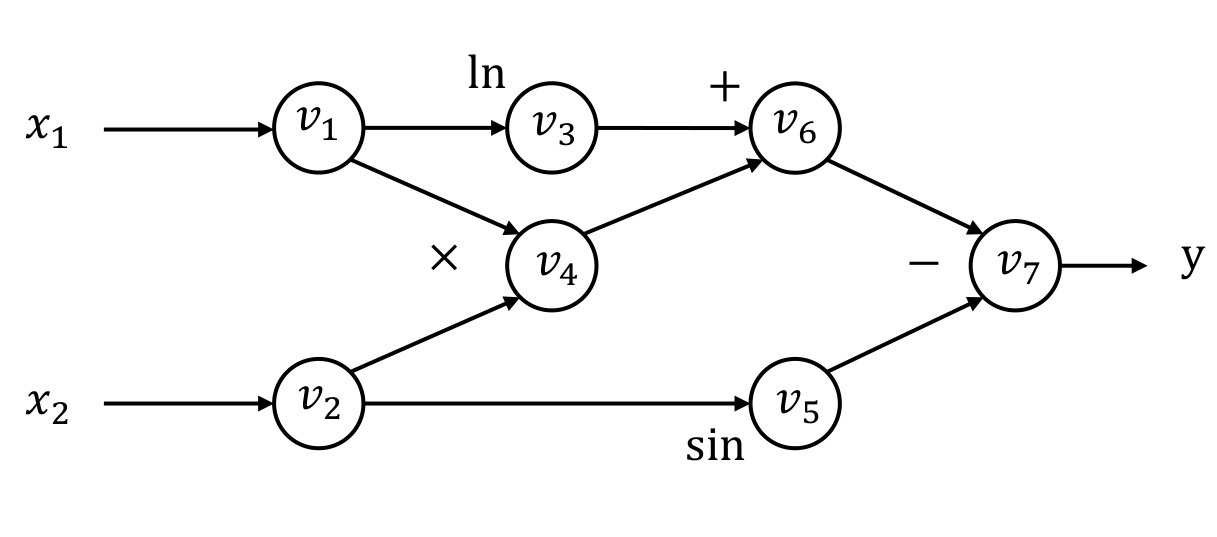
设初值
则前向计算为
forward mode AD
下面考虑在计算图上进行微分,以 为例,定义
根据微分的计算法则,有前向计算
从而
前向自动微分和 Symbolic differentiation 存在相同的问题,即可能导致一些冗余的计算
例如对于 ,为了计算 个偏导数,需要进行 轮上述过程
reverse mode AD
定义 adjoint
有反向计算
可以发现一轮反向计算可以同时计算出 和
注意到对于 的计算,其 input 都是原计算图中的顶点,所以可以将上述计算反映在原计算图中,相当于扩展了原计算图
可以多次扩展,相当于无条件的获得了计算 gradient of gradient 的能力
对于计算和扩展的时机,有两种选择
- eager,即边计算边扩展,可以一定程度上提高并行度
- lazy,即扩展完后再计算,可以通过某种方式优化计算图,提高计算效率
当然也可以不扩展,直接在原计算图上进行反向计算,这两种方法的对比如下
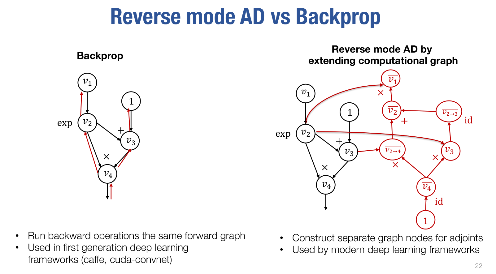
对于 backprop,可以参考第七节
5 - Automatic Differentiation Implementation
实践课
主要介绍了课程作业 needle (necessary elements of deep learning) 的架构
Key Data Structures
Value计算图中的顶点
class Value: op: Optional[Op] inputs: List["Value"] cached_data: NDArray requires_grad: boolTensor 为其子类,其中定义了大量方法以支持 Tensor 类型之间可以像原生类型那样运算,如 __add__ 和 __matmul__ 等
duck type
目前 Value 的原始数据类型为 NDArray,即 numpy.ndarray
Op顶点之间的运算
对于运算的具体实现,可以利用 array_api,或者使用其他运算 (形成计算图)
Executing the Computation
x1 = ndl.Tensor([3], dtype="float32")x2 = ndl.Tensor([4], dtype="float32")x3 = x1 * x2调用轨迹如下
autograd.TensorOp.__call__autograd.Tensor.make_from_op- 形成计算图autograd.Tensor.realize_cached_data- 进行实际的计算x3.op.compute
当开启 LAZY_MODE 时,仅会形成计算图,而不会进行实际的计算
还有一个 detach 方法,后面会提到其作用
def detach(self): """Create a new tensor that shares the data but detaches from the graph.""" return Tensor.make_const(self.realize_cached_data())hw1
Implementing forward computation
函数签名如下
def compute(self, *args: Tuple[NDArray]) -> NDArray其中
import numpy as array_apiNDArray = numpy.ndarray需要实现的 operations 有
- AddScalar
- MulScalar
- DivScalar
- PowerScalar
- EWiseAdd
- EWiseMul
- EWiseDiv
- MatMul
- Transpose
- Reshape
- BroadcastTo
- Summation
- Negate
- Log
- Exp
- ReLU
对于这些运算,只需利用 array_api,对 NDArray 原始数据对象进行计算即可
分析一下 numpy.ndarray 的表示
>>> import numpy as np>>> np.random.randn(3, 2, 1)array([[[-1.65281244], [-0.18652328]], [[-0.62980395], [-0.64332923]], [[-0.89752618], [-0.31855314]]])该 array 的 shape 为 (3, 2, 1),可以这样理解
- 最外面的一对
[],里面有 3 个元素,即[x1, x2, x3] x1里面有 2 个元素,即[y1, y2]y1里面有 1 个元素,即[z1]
分析一下几个比较特殊的运算
Summation
几乎等价于 numpy.sum,接受一个 tuple 类型的参数,代表需要进行累加的 axis
>>> a = np.arange(6).reshape(3,2,1)>>> aarray([[[0], [1]], [[2], [3]], [[4], [5]]])>>> a.sum((0,))array([[6], [9]])>>> a.sum((1,))array([[1], [5], [9]])>>> a.sum((2,))array([[0, 1], [2, 3], [4, 5]])>>> a.sum((0,1))array([15])>>> a.sum((0,2))array([6, 9])>>> a.sum((1,2))array([1, 5, 9])>>> a.sum((0,1,2))15Transpose
与 numpy.transpose 有所不同,因为 numpy.transpose 需要给出所有 axis 的位置,下标从 0 开始,例如
>>> np.random.randn(3, 2, 1).transpose().shape(1, 2, 3)>>> np.random.randn(3, 2, 1).transpose((2,1,0)).shape(1, 2, 3)>>> np.random.randn(3, 2, 1).transpose((1,2,0)).shape(2, 1, 3)这里更类似于 numpy.swapaxes,即交换两个 axis,默认为最后两个 axis
>>> np.random.randn(3, 2, 1).swapaxes(0, 1).shape(2, 3, 1)>>> np.random.randn(3, 2, 1).swapaxes(2, 0).shape(1, 2, 3)Reshape
几乎等价于 numpy.reshape,按照给定的 shape 重新布局 (with the last axis index changing fastest, back to the first axis index changing slowest),注意 flat 不变
>>> np.arange(6)array([0, 1, 2, 3, 4, 5])>>> np.arange(6).flat[2]2>>> np.arange(6).reshape((3,2))array([[0, 1], [2, 3], [4, 5]])>>> np.arange(6).reshape((3,2)).flat[2]2One shape dimension can be -1. In this case, the value is inferred from the length of the array and remaining dimensions.
BroadcastTo
几乎等价于 numpy.broadcast_to,不再赘述
MatMul
几乎等价于 numpy.matmul,这里扩展了矩阵乘法的含义,即要求 the last dimension of is not the same size as the second-to-last dimension of
>>> (np.random.randn(3, 2, 5, 4) @ np.random.randn(3, 2, 4, 6)).shape(3, 2, 5, 6)这里的 @ 运算符参考 https://peps.python.org/pep-0465/
Implementing backward computation
函数签名如下
def gradient(self, out_grad: "Value", node: "Value") -> Union["Value", Tuple["Value"]]这里的 Value 就是 Tensor 的基类
需要利用上述 operations,直接对 Tensor 进行计算,以便形成计算图
One exception is for the
ReLUoperation defined below, where you could directly access data within the Tensor without risk because the gradient itself is non-differentiable, but this is a special case.
两个要点
- the size of
out_gradwill always be the size of the output of the operation - the sizes of the
Tensorobjects returned bygradient()have to always be the same as the original inputs to the operator
由于利用数值微分检查正确性需要使用
np.linalg.norm,所以需要额外添加一个 operation 为 Sqrt,同时在添加Tensor中添加__sqrt__的定义
下面将 operations 分组进行分析
第一组,返回值类型为 "Value"
- AddScalar
- MulScalar
- DivScalar
- PowerScalar
- Negate
- Log
- Exp
- ReLU
以 PowerScalar 为例,参考公式
有
整理为代码
def gradient(self, out_grad, node): input = node.inputs[0] return self.scalar * pow(input, self.scalar - 1) * out_grad第二组,返回值类型为 Tuple["Value"]
- EWiseAdd
- EWiseMul
- EWiseDiv
采用和上述相同的方法
第三组
- MatMul
- Transpose
- Reshape
- BroadcastTo
- Summation
逐一分析这些较复杂的运算
MatMul
以二维数组为例,记
则
使用之前提到过的技巧进行计算
平衡 size
同理
若 ,上述过程可以扩展到多维数组
否则会存在 size 不匹配的情况,例如
X = np.random.randn(6, 6, 5, 4)Y = np.random.randn(4, 3)则
out_grad.shape = (6, 6, 5, 3)(out_grad @ Y.T).shape = (6, 6, 5, 4)(X.T @ out_grad).shape = (6, 6, 4, 3) != Y.shape所以需要某种方式将 shape 转换为 input 的 shape,这里考虑将多余的 axis 累加
def reverse_broadcast(x, y): # x has the shape which is broadcast from y if x.shape == y.shape: return x else: return summation(x, tuple(range(0, len(x.shape) - len(y.shape))))对于此处,相当于
summation(X.T @ out_grad, (0, 1))Transpose & Reshape
首先观察数值微分的过程
def gradient_check(f, *args, tol=1e-6, backward=False, **kwargs): eps = 1e-4 numerical_grads = [np.zeros(a.shape) for a in args] for i in range(len(args)): for j in range(args[i].realize_cached_data().size): args[i].realize_cached_data().flat[j] += eps f1 = float(f(*args, **kwargs).numpy().sum()) args[i].realize_cached_data().flat[j] -= 2 * eps f2 = float(f(*args, **kwargs).numpy().sum()) args[i].realize_cached_data().flat[j] += eps numerical_grads[i].flat[j] = (f1 - f2) / (2 * eps)相当于以 flat 的顺序逐一扰动张量的各分量,然后计算张量的各分量和
注意到这两个运算完全没有改变各分量和的大小,所以只需调整 的 size 即可,不再赘述
BroadcastTo
看几个例子找规律
np.broadcast_to(np.random.randn(3,1), (3,3))out_grad = [[1,1,1],[1,1,1],[1,1,1]]result = [[3],[3],[3]]
np.broadcast_to(np.random.randn(1,3), (3,3))out_grad = [[1,1,1],[1,1,1],[1,1,1]]result = [[3,3,3]]
np.broadcast_to(np.random.randn(1,), (3,3,3))out_grad = [[[1,1,1],[1,1,1],[1,1,1]],      [[1,1,1],[1,1,1],[1,1,1]],      [[1,1,1],[1,1,1],[1,1,1]]]result = [27]
np.broadcast_to(np.random.randn(), (3,3,3))out_grad = [[[1,1,1],[1,1,1],[1,1,1]],      [[1,1,1],[1,1,1],[1,1,1]],      [[1,1,1],[1,1,1],[1,1,1]]]result = 27
np.broadcast_to(np.random.randn(5,), (3,5))out_grad = [[1,1,1,1,1],      [1,1,1,1,1],      [1,1,1,1,1]]result = [3,3,3,3,3]
需要将 累加成 input 的 shape,分两种情况讨论
选取对应分量不同的 axis 下标构成 tuple (axes),然后进行下述运算
axes = tuple(idx for idx, axis in enumerate(input_shape) if axis == 1)return reshape(summation(out_grad, axes), input_shape)考虑化归为第一种情形,即扩展 input_shape,例如
np.broadcast_to(np.random.randn(5,), (3,5))(5,) -> (1,5)
np.broadcast_to(np.random.randn(1,), (3,3,3))(1,) -> (1,1,1)
Summation
仍然看几个例子找规律
np.random.randn(5,4).sum((1,))out_grad = [1,1,1,1,1] # (5,)result = [[1,1,1,1],[1,1,1,1],[1,1,1,1],[1,1,1,1],[1,1,1,1]]
np.random.randn(5,4).sum((0,))out_grad = [1,1,1,1] # (4,)result = [[1,1,1,1],[1,1,1,1],[1,1,1,1],[1,1,1,1],[1,1,1,1]]
np.random.randn(5,4).sum((0,1))out_grad = 1 # ()result = [[1,1,1,1],[1,1,1,1],[1,1,1,1],[1,1,1,1],[1,1,1,1]]
np.random.randn(5,4,1).sum((0,1))out_grad = [1] # (1,)result = [[[1],[1],[1],[1]],       [1],[1],[1],[1]],       [1],[1],[1],[1]],       [1],[1],[1],[1]],       [1],[1],[1],[1]]]
需要将 广播成 input 的 shape
某种意义上 Summation 运算和 BroadcastTo 运算互为逆运算
若 self.axes 为 None,则 为标量,直接广播即可
否则,需要先对 进行 reshape,使其接近 input 的 shape,对于上面几个例子
np.random.randn(5,4).sum((1,))out_grad.reshape((5,1))
np.random.randn(5,4).sum((0,))out_grad.reshape((1,4))
np.random.randn(5,4,1).sum((0,1))out_grad.reshape((1,1,1))
然后再进行广播
Topological sort
给定一个计算图的终点,计算其拓扑排序,例如
a1, b1 = ndl.Tensor(np.asarray([[0.88282157]])), ndl.Tensor(np.asarray([[0.90170084]]))c1 = 3*a1*a1 + 4*b1*a1 - a1topo_order = np.array([x.numpy() for x in ndl.autograd.find_topo_sort([c1])])则 topo_order 应为 [a1, ..., c1]
注意一幅有向无环图的拓扑顺序即为所有顶点的逆后序排序,又因为这里给出了终点,所以直接后序遍历即可
Implementing reverse mode differentiation
以 为例,其对应的计算图和扩展的计算图如下

下面使用文字描述扩展计算图的过程
- 以逆拓扑排序的顺序遍历原计算图的每个顶点
- 对于每个顶点
- 通过其出边计算出该顶点的 gradient
- 遍历该顶点的入边,计算对应的 backward gradient,并保存起来
使用伪代码将上述算法描述如下
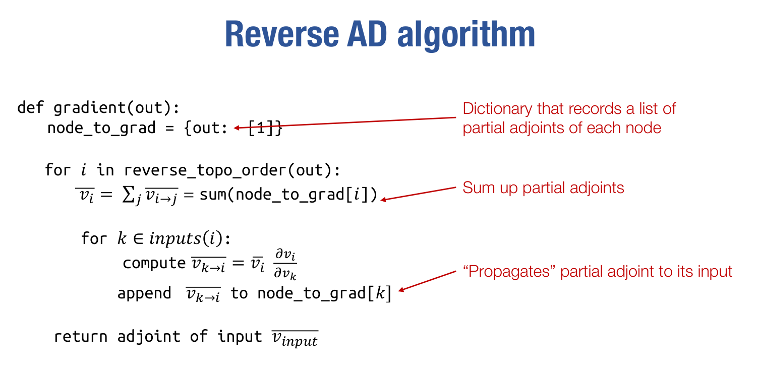
其中
在实际的作业中,需要关注两点
- 计算图的扩展,对应发生在 和计算各入边的 backward gradient
计算各入边的 backward gradient 就是通过 gradient 函数实现的,其中已经利用 operations 直接对 Tensor 进行了计算
所以只需考虑利用 operations 计算
- 各顶点的 gradient 保存在变量
grad中
Softmax loss
类似 hw0 里面的 softmax_loss,但是参数的类型和含义发生了变化
首先参数类型变为了 Tensor,然后 y 的含义如下
X, y = parse_mnist(...)y_one_hot = np.zeros((y.shape[0], 10))y_one_hot[np.arange(y.size), y] = 1y = ndl.Tensor(y_one_hot)也就是 y 的 shape 为 (batch, num_classes)
类似之前的
可以认为这里的 softmax_loss 是一个新的 operation,所以其计算需要使用之前的那些 operations,直接对 Tensor 进行计算,以便形成计算图
def softmax_loss(Z, y_one_hot): batch_size = Z.shape[0] return (ndl.summation(ndl.log(ndl.summation(ndl.exp(Z), axes=(1,)))) - ndl.summation(Z * y_one_hot)) / batch_size注意此处 Summation 运算的使用,最后的结果为一个标量值,仍然为 Tensor 类型
SGD for a two-layer neural network
类似 hw0 里面的 nn_epoch
对于每一次迭代,需要使用之前的那些 operations 构造出 loss
X_batch = X[batch * i: batch * (i + 1)]y_batch = y[batch * i: batch * (i + 1)]
Z1 = ndl.Tensor(X_batch) @ W1Z2 = ndl.relu(Z1) @ W2
y_one_hot = np.zeros((batch, num_classes))y_one_hot[np.arange(y_batch.size), y_batch] = 1y_one_hot = ndl.Tensor(y_one_hot)
loss = softmax_loss(Z2, y_one_hot)
然后对 loss 调用 backward 自动微分
根据上面的分析,此时 W1 和 W2 的 gradient 就已经保存在变量 grad 中了,此处只需根据公式更新即可
W1 = (W1 - lr * ndl.Tensor(W1.grad)).detach()W2 = (W2 - lr * ndl.Tensor(W2.grad)).detach()注意此处的 detach,避免在多次迭代中计算图膨胀,耗尽内存
可能更好的写法
原地更新 W1 和 W2,避免重新构造
Tensor
6 - Optimization
Gradient descent
其中 代表整个需要优化的公式
注意区分这里的 和带下标的 ,不带下标的版本代表对参数 求梯度,带下标的 代表第 次迭代后参数的值
不同的学习率会带来不同的效果,以二次函数为例
其中 为 positive definite (all positive eigenvalues)

Newton’s Method
其中 为黑塞 (Hessian) 矩阵,即二阶偏导数构成的方阵
注意这里都是逐元素运算
对于上述二次函数,取 可以直接得到极值

二阶偏导给出了极值的准确方向
但是由于黑塞矩阵计算量巨大,且绝大部分模型没有二次函数那么简单,所以在实践中运用不多
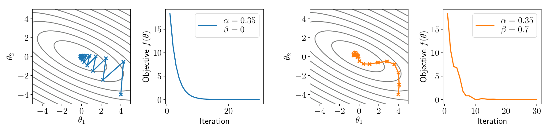
Momentum
考虑之前迭代的累计效果
其中 为另一个超参数,当 时,即退化为 Gradient descent
Bias correction term
考虑展开
会发现 will be smaller in initial iterations than in later ones
引入 bias correction term,即
后面 Adam 也存在类似的操作
引入后的结果对比

Nesterov Momentum
Momentum 的一个变体,不太理解
Adam
引入两个超参数
注意这里都是逐元素运算
也可以引入 bias correction term,具体参考 hw2

Stochastic variants
贴原文,不太理解,大概是区分 batch 和 minibatch
All the previous examples considered batch update to the parameters, but the single most important optimization choice is to use stochastic variants.
We can get a noisy (but unbiased) estimate of gradient by computing gradient of the loss over just a subset of examples (called a minibatch).
Instead of taking a few expensive, noise-free, steps, we take many cheap, noisy steps, which ends having much strong performance per compute.
7 - Neural Network Library Abstractions
Case studies
Forward and backward layer interface (Caffe 1.0)
Defines the forward computation and backward (gradient) operations
class Layer: def forward(bottom, top): pass def backward(top, propagate_down, bottom): pass- 直接在原计算图上进行反向计算
- 使 gradient computation 和 module composition 产生了耦合
Computational graph and declarative programming (Tensorflow 1.0)
First declare the computational graph, then execute the graph by feeding input value
import tensorflow as tf
v1 = tf.Variable()v2 = tf.exp(v1)v3 = v2 + 1v4 = v2 * v3
sess = tf.Session()value4 = sess.run(v4, feed_dict={v1: numpy.array([1])})- 便于优化
- Session 机制可以让实际的运算在远程进行或分布式进行
Imperative automatic differentiation (PyTorch)
Executes computation as we construct the computational graph
import needle as ndl
v1 = ndl.Tensor([1])v2 = ndl.exp(v1)v3 = v2 + 1v4 = v2 * v3if v4.numpy() > 0.5:  v5 = v4 * 2else:  v5 = v4
v5.backward()- 方便调试 (如打印节点的值),增加易用性
- 可以使用高级编程语言的控制流机制,描述更加复杂的计算图
needle 便采用了这种方案
High level modular library components

8 - NN Library Implementation
实践课
Designing a Neural Network Library
简化版的 hw2,基于 hw1
class Parameter(ndl.Tensor):    """parameter"""
def _get_params(value):    if isinstance(value, Parameter):        return [value]    if isinstance(value, dict):        params = []        for k, v in value.items():            params += _get_params(v)        return params    if isinstance(value, Module):        return value.parameters()    return []
class Module:    def parameters(self):        return _get_params(self.__dict__)
    def __call__(self, *args, **kwargs):        return self.forward(*args, **kwargs)
class ScaleAdd(Module):    def __init__(self, init_s=1, init_b=0):        self.s = Parameter([init_s], dtype="float32")        self.b = Parameter([init_b], dtype="float32")
    def forward(self, x):        return x * self.s + self.b
class MultiPathScaleAdd(Module):    def __init__(self):        self.path0 = ScaleAdd()        self.path1 = ScaleAdd()
    def forward(self, x):        return self.path0(x) + self.path1(x)
class L2Loss(Module):    def forward(self, x ,y):        z = x + (-1) * y        return z * z
class Optimizer:    def __init__(self, params):        self.params = params
    def reset_grad(self):        for p in self.params:            p.grad = None
    def step(self):        raise NotImplemented()
class SGD(Optimizer):    def __init__(self, params, lr):        self.params = params        self.lr = lr
    def step(self):        for w in self.params:            w.data = w.data + (-self.lr) * w.grad
x = ndl.Tensor([2], dtype="float32")y = ndl.Tensor([2], dtype="float32")
model = MultiPathScaleAdd()l2loss = L2Loss()opt = SGD(model.parameters(), lr=0.01)num_epoch = 10
for epoch in range(num_epoch):    opt.reset_grad()    h = model(x)    loss = l2loss(h, y)    training_loss = loss.numpy()    loss.backward()    opt.step()
    print(training_loss)
Fused operator and Tuple Value
Up until now each of the needle operator only returns a single output Tensor. In real world application scenarios, it is somtimes helpful to compute many outputs at once in a single (fused) operator.
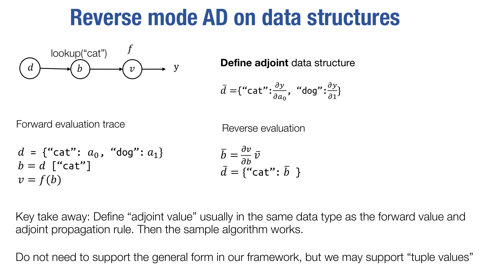
Needle is designed to support this feature. In order to do so, we need to introduce a new kind of Value.
autograd.py: TheTensorTupleclassops.py:TupleGetItemandMakeTensorTuple
对于这种复杂的数据结构,仍然可以定义其 adjoint value,例如第四节课件的最后一页
9 - Initialization, Normalization and Regularization
Initialization
主要参考了《深度学习入门》第 6.2 节
可以将权重初始值设为 0 吗
为什么不能将权重初始值设为 0 呢?严格地说,为什么不能将权重初始值设成一样的值呢?这是因为在误差反向传播法中,所有的权重值都会进行相同的更新。比如,在 2 层神经网络中,假设第 1 层和第 2 层的权重为 0。这样一来,正向传播时,因为输入层的权重为 0,所以第 2 层的神经元全部会被传递相同的值。第 2 层的神经元中全部输入相同的值,这意味着反向传播时第 2 层的权重全部都会进行相同的更新。因此,权重被更新为相同的值,并拥有了对称的值(重复的值)。这使得神经网络拥有许多不同的权重的意义丧失了。为了防止『权重均一化』(严格地讲,是为了瓦解权重的对称结构),必须随机生成初始值。
Xavier 初始值
如果前一层的节点数为 ,则初始值使用标准差为 的高斯分布
ReLU 的权重初始值
如果前一层的节点数为 ,则初始值使用标准差为 的高斯分布
不严格的说明如下
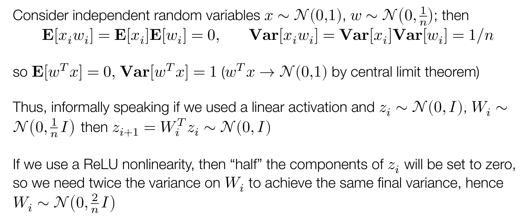
如果系数不对,会出现如下现象
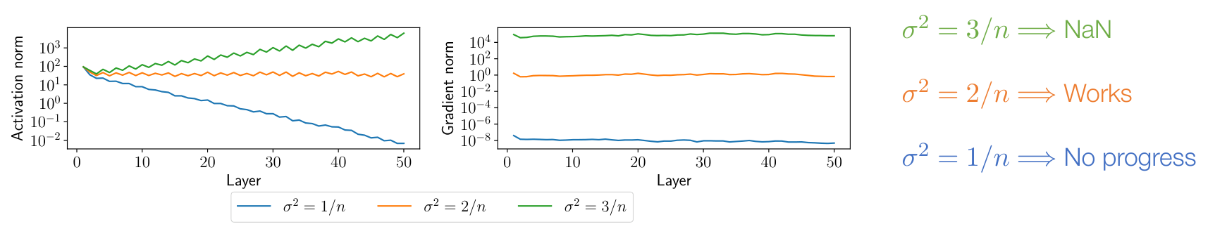
- 若方差为 ,激活值 (activation value) 会减少,梯度偏小,学习几乎无进展
- 若方差为 ,激活值 (activation value) 会增加,梯度偏大,会出现浮点溢出
激活值就是每一层 的值
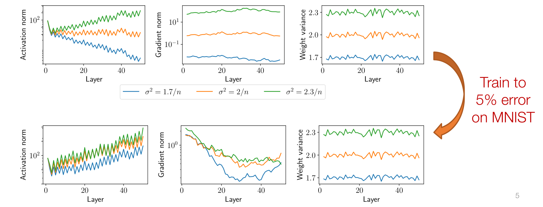
即使训练成功完成了,在训练过程中权重的变化可能也不会太大,这强调了权重初始值的意义
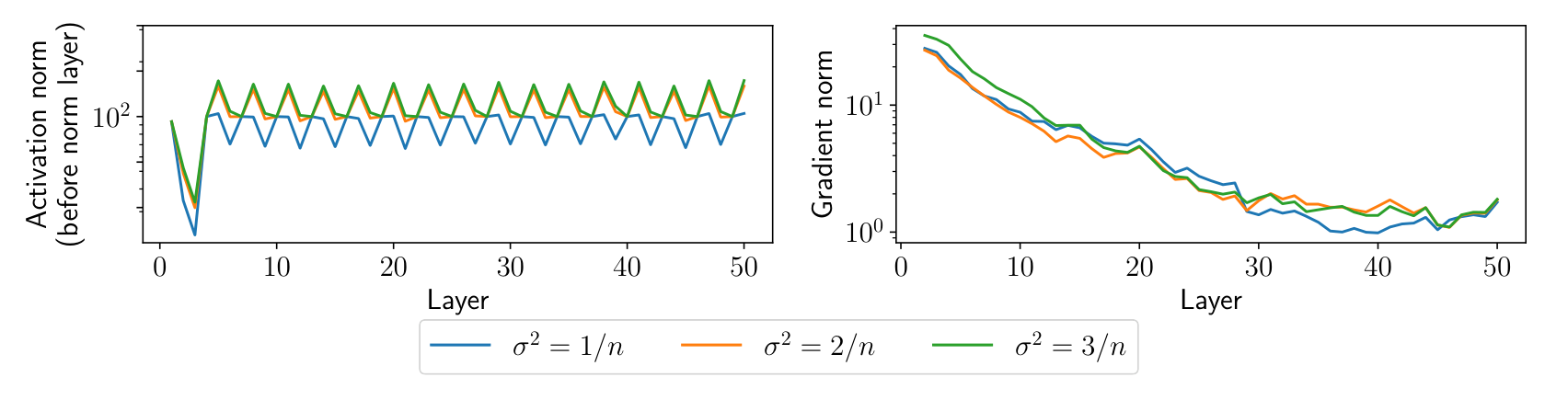
Normalization
Normalization 的意义在于让激活值在层与层之间保持相同的分布,如高斯分布
Layer normalization
让激活值保持标准正态分布
此处 是为了避免除零异常
效果如下
Batch normalization
在某些情形中,激活值的分布特征也可能是一个有用的 discriminative feature
在 batch 形式下,Layer normalization 相当于按行 normalize,我们考虑按列 normalize
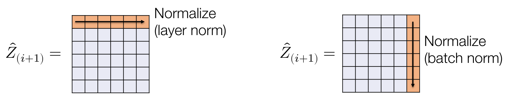
然而在推理 (inference) 过程中,使用 Batch normalization 会导致激活值依赖于选取的 batch,也就是不同的样本之间产生了依赖关系,所以

具体参考 hw2
inference / test / evaluation
Regularization
通常情况下,神经网络的参数空间维度是大于真实的数据空间维度的,所以在某种意义上,神经网络可以完全拟合训练的数据,这就会导致过拟合,泛化能力偏弱
为了避免过拟合,考虑限制神经网络的复杂度,通常有两种做法
- Implicit regularization refers to the manner in which our existing algorithms (namely SGD) or architectures already limit functions considered
E.g., we aren’t actually optimizing over “all neural networks”, we are optimizing over all neural networks considered by SGD, with a given weight initialization
- Explicit regularization refers to modifications made to the network and training procedure explicitly intended to regularize the network
下面主要讨论 Explicit regularization
L2 Regularization (weight decay)
主要思想是使权重保持在一个比较小的值,这样函数会『平滑』一些
为此添加正则项
则权重的更新公式为
Dropout
主要思想是随机将激活层的某些分量置为零
此处除以 是为了保持均值不变
Dropout as stochastic approximation - instructive to consider Dropout as bringing a similar stochastic approximation as SGD to the setting of individual activations
Takeaway message
I don’t want to give the impression that deep learning is all about random hacks: there have been a lot of excellent scientific experimentation with all the above.
But it is true that we don’t have a complete picture of how all the different empirical tricks people use really work and interact.
业界对于 Batch normalization 的原理尚无定论
The “good” news is that in many cases, it seems to be possible to get similarly good results with wildly different architectural and methodological choices.
Batch normalization 对于 out-of-distribution data (例如对图像进行某些变换) 的 inference 可以提供帮助
hw2
setup
使用 PyCharm 打开项目时,需要在 Project Structure 里面配置好 Source Folders

否则 PyCharm 会认为项目的根目录为 root,在这种情况下,为了能够正确的跳转,需要修改一些 import 语句,如修改
import needle为
import python.needle这可能导致符号的 duplication,例如同时出现 needle.autograd.Tensor 和 python.needle.autograd.Tensor,虽然这两个符号所代指的类型是一致的,但是 Python 会在两个内存区域存储这些 type,从而导致某些类型检查失败,如
assert isinstance(value, Tensor)所以不应该修改 import 语句,而应该配置好 Source Folders
weight initialization
注意这里权重初始化的 shape 为
Xavier
Understanding the difficulty of training deep feedforward neural networks
- uniform
- normal
Kaiming
Delving deep into rectifiers: Surpassing human-level performance on ImageNet classification
Use the recommended gain value for ReLU:
- uniform
- normal
operator
LogSumExp
由于需要实现 stable 的 LogSumExp 运算,所以需要利用 numpy.amax,其语义如下
>>> a = np.arange(6).reshape(3,2,1)>>> aarray([[[0], [1]], [[2], [3]], [[4], [5]]])>>> a.max((0,))array([[4], [5]])>>> a.max((1,))array([[1], [3], [5]])>>> a.max((2,))array([[0, 1], [2, 3], [4, 5]])>>> a.max((0,1))array([5])>>> a.max((0,2))array([4, 5])>>> a.max((1,2))array([1, 3, 5])>>> a.max((0,1,2))5下面考虑 LogSumExp 运算
由于经过 max 运算后, 的 shape 和 的 shape 会不一致,例如
ops.logsumexp(np.random.randn(3,3,3), axes=(1,2))Z.shape = (3,3,3)Z_max.shape = (3,)所以需要进行 reshape 和 broadcast 运算,使 的 shape 变换为 的 shape
对于 backward 运算,其核心部分如下,不太理解
Z_max_ori = broadcast_to(reshape(Z_max, reshape_shape), Z.shape)Z_exp = exp(Z - Z_max_ori)sum_exp = broadcast_to(reshape(summation(Z_exp, self.axes), reshape_shape), Z.shape)out_grad = broadcast_to(reshape(out_grad, reshape_shape), Z.shape)return out_grad * Z_exp / sum_expmodules
Linear
约定
input.shape = (N, in)output.shape = (N, out)参考 issues,设置 bias 的 shape 为 (out,),注意需要对应修改测试用例 test_nn_linear_bias_init_1
ReLU
直接利用 ReLU 运算
Sequential
复合应用多个 modules
SoftmaxLoss
利用 LogSumExp 运算
配合使用 init.one_hot
LayerNorm1d
这里期望和方差是按行意义上的
约定
x.shape = (batch_size, dim)Flatten
(B, X_0, X_1, ...) -> (B, X_0 * X_1 * ...)BatchNorm1d
Batch Normalization: Accelerating Deep Network Training by Reducing Internal Covariate Shift
这里期望和方差是按列意义上的
在 inference 阶段,使用在 train 阶段记录的 running estimates of mean and variance
这里期望和方差仍然是按列意义上的
其中 为 momentum
仍然约定
x.shape = (batch_size, dim)Dropout
Improving neural networks by preventing co-adaption of feature detectors
dropout 只能发生在 train 阶段
配合使用 init.randb
Residual
input: module and Tensor
output:
optimizers
SGD
包含 momentum 超参数和 weight decay (L2 penalty)
注意不可以直接使用下述形式,因为有 momentum 项
Adam
Adam: A Method for Stochastic Optimization
下述写法会导致 test_optim_adam_z_memory_check_1 失败,注意到 grad 已经 detached 了,没有必要添加多余的 .data 调用
def step(self): ### BEGIN YOUR SOLUTION self.t += 1 for param in self.params: grad = param.grad.data + self.weight_decay * param.data grad = ndl.Tensor(grad.data, dtype='float32') self.m[param] = (self.beta1 * self.m.get(param, 0) + (1 - self.beta1) * grad).data self.v[param] = (self.beta2 * self.v.get(param, 0) + (1 - self.beta2) * grad * grad).data m_hat = self.m[param] / (1 - self.beta1 ** self.t) v_hat = self.v[param] / (1 - self.beta2 ** self.t) param.data -= self.lr * m_hat / (ndl.ops.sqrt(v_hat) + self.eps) ### END YOUR SOLUTIONdata primitives
Transformations
注意这里的
C在最内层,代表 number of channels of the image
RandomFlipHorizontal
shape 为 H x W x C
利用 numpy.flip 即可
RandomCrop
shape 为 H x W x C
利用 numpy.pad 和索引即可
Dataset
Dataset stores the samples and their corresponding labels
需要实现 MNISTDataset,其 samples 和 labels 的原始 shape 为
X.shape = (60000, 28 * 28)y.shape = (60000,)通过 index 索引到对应的 sample 后,需要 reshape 为 (-1, 28, 28, 1),即 NHWC 格式,以便传入 transforms 进行变换
这里的 index 可能是一个列表
Dataloader
DataLoader wraps an iterable around the Dataset to enable easy access to the samples
其中使用了 numpy.array_split 作为索引
>>> np.array_split(np.arange(100), range(10, 100, 10))[array([0, 1, 2, 3, 4, 5, 6, 7, 8, 9]), array([10, 11, 12, 13, 14, 15, 16, 17, 18, 19]), array([20, 21, 22, 23, 24, 25, 26, 27, 28, 29]), array([30, 31, 32, 33, 34, 35, 36, 37, 38, 39]), array([40, 41, 42, 43, 44, 45, 46, 47, 48, 49]), array([50, 51, 52, 53, 54, 55, 56, 57, 58, 59]), array([60, 61, 62, 63, 64, 65, 66, 67, 68, 69]), array([70, 71, 72, 73, 74, 75, 76, 77, 78, 79]), array([80, 81, 82, 83, 84, 85, 86, 87, 88, 89]), array([90, 91, 92, 93, 94, 95, 96, 97, 98, 99])]修改了 test_dataloader_mnist 这个测试用例,batch_size 是否为 1 应该不影响代码一致性,因为索引都是 List 类型
for i, batch in enumerate(mnist_train_dataloader): batch_x, batch_y = batch[0].numpy(), batch[1].numpy() truth = mnist_train_dataset[i * batch_size: (i + 1) * batch_size] truth_x = truth[0] truth_y = truth[1]此处 batch 类型为 List[Tensor],有如下关系
batch[0].shape = (batch_size, 28, 28, 1)batch[1].shape = (batch_size,)truth 类型为 List[numpy.ndarray],shape 与上述一致
put it all together
ResidualBlock
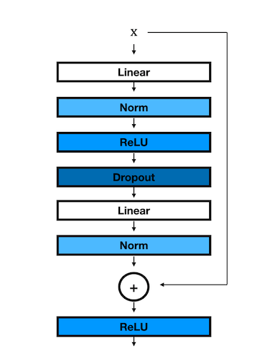
返回一个新的 module
MLPResNet

返回一个新的 module (model)
Epoch
类似 hw0 里面的 nn_epoch
Train Mnist
- 使用 MNIST 数据集构造
DataLoader - model 为 MLPResNet
- optimizer 为 Adam
Result
对于测试用例 test_mlp_train_mnist_1,由于虚拟机内存不够
██████████████████ ████████ vgalaxy@vgalaxy-virtualbox ██████████████████ ████████ OS: Manjaro 22.0.0 Sikaris ██████████████████ ████████ Kernel: x86_64 Linux 5.15.81-1-MANJARO ██████████████████ ████████ Uptime: 12m ████████ ████████ Packages: 1334 ████████ ████████ ████████ Shell: zsh 5.9 ████████ ████████ ████████ Resolution: 1920x964 ████████ ████████ ████████ DE: GNOME 43.1 ████████ ████████ ████████ WM: Mutter ████████ ████████ ████████ WM Theme: ████████ ████████ ████████ GTK Theme: Adw-dark [GTK2/3] ████████ ████████ ████████ Icon Theme: Papirus-Dark ████████ ████████ ████████ Font: Noto Sans 11 ████████ ████████ ████████ Disk: 32G / 84G (40%) CPU: Intel Core i7-10875H @ 8x 2.304GHz GPU: llvmpipe (LLVM 14.0.6, 256 bits) RAM: 3163MiB / 10959MiB会出现
Process finished with exit code 137 (interrupted by signal 9: SIGKILL)于是考虑调整参数,对于
train_mnist(batch_size=200, epochs=1, hidden_dim=50, data_dir="../data")结果为
(train_error, train_loss, test_error, test_loss) = (0.19863333333333333, 0.6607103530247999, 0.0706, 0.24144852809906003)由于 epochs 和 hidden_dim 设置的较小,所以还有很大的提升空间
11 - Hardware Acceleration
General acceleration techniques
Vectorization
adding two arrays of length 256
void vecadd(float* A, float *B, float* C) { for (int i = 0; i < 64; ++i) { float4 a = load_float4(A + i*4); float4 b = load_float4(B + i*4); float4 c = add_float4(a, b); store_float4(C + i*4, c); }}memory (A, B, C) needs to be aligned to 128 bits
Data layout and strides
- Row major (C)
A[i, j] => Adata[i * A.shape[1] + j]- Column major (Fortran)
A[i, j] => Adata[j * A.shape[0] + i]- Strides format
A[i, j] => Adata[i * A.strides[0] + j * A.strides[1]]其中的 strides 选取特定的值即可转换为 Row major 或 Column major
Discussion about strides
Advantages: can perform transformation / slicing in zero copy way
- Slice: change the begin offset and shape
- Transpose: swap the strides
- Broadcast: insert a stride equals 0
Disadvantages: memory access becomes not continuous
- Makes vectorization harder
- Many linear algebra operations may require compact the array first
第十三节会通过例子描述 strides 的意义
Parallelization
以 OpenMP 为例
void vecadd(float* A, float *B, float* C) { #pragma omp parallel for for (int i = 0; i < 64; ++i) { float4 a = load_float4(A + i*4); float4 b = load_float4(B + i*4); float4 c = add_float4(a, b); store_float4(C * 4, c); }}Executes the computation on multiple threads
Case study: matrix multiplication
计算
其中
下面考虑方阵的情形
Vanilla matrix multiplication
dram float A[n][n], B[n][n], C[n][n];
for (int i = 0; i < n; ++i) {  for (int j = 0; j < n; ++j) {    register float c = 0;    for (int k = 0; k < n; ++k) {      register float a = A[i][k];      register float b = B[j][k];      c += a * b;    }    C[i][j] = c;  }}
其中 dram (DRAM) 和 register 代表了数据所处的内存层级
下面计算内存开销
- A’s dram -> register time cost:
n^3 - B’s dram -> register time cost:
n^3 - A’s register memory cost:
1 - B’s register memory cost:
1 - C’s register memory cost:
1
总结为
- Load cost:
2 * dramspeed * n^3 - Register cost:
3
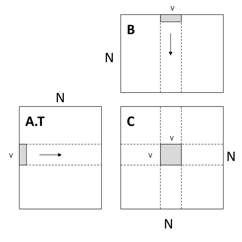
Register tiled matrix multiplication
考虑使用更多的 registers 以减少 load 的次数
dram float A[n / v1][n / v3][v1][v3];dram float B[n / v2][n / v3][v2][v3];dram float C[n / v1][n / v2][v1][v2];
for (int i = 0; i < n / v1; ++i) {  for (int j = 0; j < n / v2; ++j) {    register float c[v1][v2] = 0;    for (int k = 0; k < n / v3; ++k) {      register float a[v1][v3] = A[i][k];      register float b[v2][v3] = B[j][k];      c += dot(a, b.T);    }    C[i][j] = c;  }}
代码中有些部分进行了简化,具体可以参考 hw3
示意图如下

下面计算内存开销
- A’s dram -> register time cost:
n^3/v2 - B’s dram -> register time cost:
n^3/v1 - A’s register memory cost:
v1*v3 - B’s register memory cost:
v2*v3 - C’s register memory cost:
v1*v2
总结为
- Load cost:
dramspeed * (n^3/v2 + n^3/v1) - Register cost:
v1*v3 + v2*v3 + v1*v2
Cache line aware tiling
考虑引入 L1 Cache 这一内存层级,加速内存访问
dram float A[n / b1][b1][n];dram float B[n / b2][b2][n];dram float C[n / b1][n / b2][b1][b2];
for (int i = 0; i < n / b1; ++i) {  l1cache float a[b1][n] = A[i];  for (int j = 0; j < n / b2; ++j) {    l1cache float b[b2][n] = B[j];    C[i][j] = dot(a, b.T);  }}
其中 dot 即为上述 register tiled matrix multiplication
示意图如下
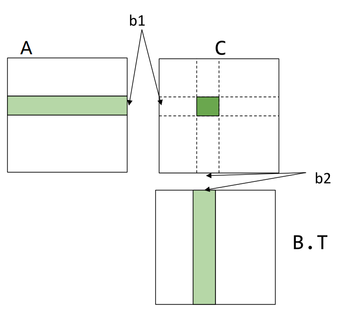
下面计算内存开销
- A’s dram -> l1 cache time cost:
(n/b1)*(n*b1)=n^2 - B’s dram -> l1 cache time cost:
(n/b1)*(n/b2)*(n*b2)=n^3/b1
有一些约束条件
b1 * n + b2 * n小于 L1 Cache 的大小b1 % v1 == 0且b2 % v2 == 0
Putting it together
dram float A[n / b1][b1 / v1][n][v1];dram float B[n / b2][b2 / v2][n][v2];
for (int i = 0; i < n / b1; ++i) {  l1cache float a[b1 / v1][n][v1] = A[i];  for (int j = 0; j < n / b2; ++j) {    l1cache float b[b2 / v2][n][v2] = B[j];    for (int x = 0; x < b1 / v1; ++x)      for (int y = 0; y < b2 / v2; ++y) {        register float c[v1][v2] = 0;        for (int k = 0; k < n; ++k) {          register float ar[v1] = a[x][k][:];          register float br[v2] = b[y][k][:];          C += dot(ar, br.T)        }      }  }}
Load cost 总结为 l1speed * (n^3/v2 + n^3/v1) + dramspeed * (n^2 + n^3/b1)
12 - GPU Acceleration
GPU programming
以 cuda 为例
GPU programming mode: SIMT
- Single instruction multiple threads (SIMT)
- All threads executes the same code, but can take different path
- Threads are grouped into blocks
- Thread within the same block have shared memory
- Blocks are grouped into a launch grid
- A kernel executes a grid
GPU memory hierarchy

可以通过 shared memory 减少 load 的次数,下面会具体介绍
Example: vector add
不多解释了
// device side__global__ void VecAddKernel(float* A, float* B, float* C, int n) {  int i = blockDim.x * blockIdx.x + threadIdx.x;  if (i < n) {    C[i] = A[i] + B[i];  }}
// host sidevoid VecAddCUDA(float* Acpu, float* Bcpu, float* Ccpu, int n) {  float *dA, *dB, *dC;  cudaMalloc(&dA, n * sizeof(float));  cudaMalloc(&dB, n * sizeof(float));  cudaMalloc(&dC, n * sizeof(float));  cudaMemcpy(dA, Acpu, n * sizeof(float), cudaMemcpyHostToDevice);  cudaMemcpy(dB, Bcpu, n * sizeof(float), cudaMemcpyHostToDevice);  int threads_per_block = 512;  int nblocks = (n + threads_per_block - 1) / threads_per_block;  VecAddKernel<<<nblocks, thread_per_block>>>(dA, dB, dC, n);  cudaMemcpy(Ccpu, dC, n * sizeof(float), cudaMemcpyDeviceToHost);  cudaFree(dA);  cudaFree(dB);  cudaFree(dC);}
Case study: matrix multiplication on GPU
计算
其中
与上一节略有不同
下面考虑方阵的情形
Thread-level: register tiling
每个 thread 负责计算一块 的区域,临时数据存储在 register 中
__global__ void mm(float A[N][N], float B[N][N], float C[N][N]) { int ybase = blockIdx.y * blockDim.y + threadIdx.y; int xbase = blockIdx.x * blockDim.x + threadIdx.x; float c[V][V] = {0}; float a[V], b[V]; for (int k = 0; k < N; ++k) { a[:] = A[k, ybase * V: ybase * V + V]; b[:] = B[k, xbase * V: xbase * V + V]; for (int y = 0; y < V; ++y) { for (int x = 0; x < V; ++x) { c[y][x] += a[y] * b[x]; } } } C[ybase * V: ybase * V + V, xbase * V: xbase * V + V] = c[:];}示意图如下
Block-level: shared memory tiling
每个 thread block 负责计算一块 的区域,其中的每个 thread 负责其中的一块 的区域
thread block 预先为输入数据在 block shared memory 中分配内存
__global__ void mm(float A[N][N], float B[N][N], float C[N][N]) { __shared__ float sA[S][L], sB[S][L]; float c[V][V] = {0}; float a[V], b[V]; int yblock = blockIdx.y; int xblock = blockIdx.x; for (int ko = 0; ko < N; ko += S) { __syncthreads(); // needs to be implemented by thread cooperative fetching sA[:, :] = A[k: k + S, yblock * L: yblock * L + L]; sB[:, :] = B[k: k + S, xblock * L: xblock * L + L]; __syncthreads(); for (int ki = 0; ki < S; ++ki) { a[:] = sA[ki, threadIdx.y * V: threadIdx.y * V + V]; b[:] = sB[ki, threadIdx.x * V: threadIdx.x * V + V]; for (int y = 0; y < V; ++y) { for (int x = 0; x < V; ++x) { c[y][x] += a[y] * b[x]; } } } } int ybase = blockIdx.y * blockDim.y + threadIdx.y; int xbase = blockIdx.x * blockDim.x + threadIdx.x; C[ybase * V: ybase * V + V, xbase * V: xbase * V + V] = c[:];}对于
实际上应该展开为
示意图如下

下面分析其内存开销
- global -> shared:
2 * N^3/L - shared -> register:
2 * N^3/V
More GPU optimization techniques
Checkout CUDA Programming guide
- Global memory continuous read
- Shared memory bank conflict
- Software pipelining
- Warp level optimizations
- Tensor Core
13 - Hardware Acceleration Implementation
实践课
这一节的目标是构建高性能的 NDArray 库
在此之前,array_api 和 NDArray 的定义是通过 numpy 导出的
import numpy as array_apiNDArray = numpy.ndarray在构建完 NDArray 库后,可以通过如下的方式定义
from . import backend_ndarray as array_apiNDArray = array_api.NDArrayKey Data Structures
backend_ndarray 模块的主要内容在 ndarray.py 中,其核心数据结构如下
NDArray: the container to hold device specific ndarrayBackendDevice: backend device- mod holds the module implementation that implements all functions
目前支持三种 devices
cpu_numpy,定义在ndarray_backend_numpy.py中,本质是通过 numpy 实现的,可以作为下述 devices 的参考实现cpu,定义在ndarray_backend_cpu.cc中,使用 C++ 实现,可以考虑引入 OpenMP 加速gpu,定义在ndarray_backend_cuda.cu中,使用 C++ 和 CUDA 实现
后面两种 devices 的内部符号通过 pybind11 这个第三方库导出到 Python 中,例如
PYBIND11_MODULE(ndarray_backend_cpu, m) {  namespace py = pybind11;  using namespace needle;  using namespace cpu;
  m.attr("__device_name__") = "cpu";
  py::class_<AlignedArray>(m, "Array")      .def(py::init<size_t>(), py::return_value_policy::take_ownership)      .def("ptr", &AlignedArray::ptr_as_int)      .def_readonly("size", &AlignedArray::size);
  m.def("from_numpy", [](py::array_t<scalar_t> a, AlignedArray *out) {    std::memcpy(out->ptr, a.request().ptr, out->size * ELEM_SIZE);  });
  ...}
相当于使用 Python 定义了下述符号
__device_name__ = "cpu"
class Array:    pass
def from_numpy(a, out):    pass
...
NDArray Data Structure
An NDArray contains the following fields
handle: The backend handle that build a flat array which stores the datashape: The shape of the NDArraystrides: The strides that shows how do we access multi-dimensional elementsoffset: The offset of the first elementdevice: The backend device that backs the computation
其中 (shape, strides, offset) 这三个字段起到视图的作用,在 hw3 中会详细解释
device 字段指向一个 BackendDevice 对象
实际的数据存储在 handle 这个字段中,本质上是一段连续的内存,内存的分配仅会在 NDArray.make 这个静态方法中进行
这里需要引入一个重要的概念 compact,其定义如下
def is_compact(self): """Return true if array is compact in memory and internal size equals product of the shape dimensions""" return ( self._strides == self.compact_strides(self._shape) and prod(self.shape) == self._handle.size )这里似乎并没有考虑
offset字段
上述定义等价于,在视图作用下,其内存访问的顺序是 row major 的
为了简化 device 端的代码,一般情况下,其传入的底层数据都是 compacted 的,并且已经分配好了内存
除了 compact 和 setitem 操作,详见 hw3
hw3
Python array operations
下述运算不需要修改底层存储的数据,只需要修改其视图即可
- shape
- strides
- offset
所以使用 Python 语言实现
reshape
对于 compact stride 的计算
def compact_strides(shape): """ Utility function to compute compact strides """ stride = 1 res = [] for i in range(1, len(shape) + 1): res.append(stride) stride *= shape[-i] return tuple(res[::-1])例如
compact_strides((4,3,2)) == (6,2,1)考虑 shape dimension 中存在 -1 的情形
permute
几乎等价于 numpy.transpose
考虑 index 为负数的情形,暂不考虑 axes 为 None 的情形
根据 new_axes 调整 shape 和 strides 即可
new_shape = tuple([self.shape[i] for i in new_axes])new_strides = tuple([self.strides[i] for i in new_axes])broadcast_to
扩展 shape 和 strides,使其 ndim 与 new_shape 一致
然后 shape 为 1 的 dimension 其对应的 stride 置 0 即可
getitem
根据 (start, stop, step) 构造 shape, strides, offset 即可
One thing to note is that the
__getitem__()call, unlike numpy, will never change the number of dimensions in the array. So e.g., for a 2D NDArrayA,A[2,2]would return a still-2D with one row and one column. And e.g.A[:4,2]would return a 2D NDarray with 4 rows and 1 column.
因为上述原因,所以测试用例中不能出现某个维度只返回一个元素的情形
另外参考 issues,修改
start = self.shape[dim]为
start = self.shape[dim] + start以支持合理的负数索引
CPU Backend - Compact and setitem
实现下面三个操作
CompactEwiseSetitemScalarSetitem
假设 out 为 compacted 的,in 进行了上述某些变换,则 Compact 的核心操作如下
IndicesGenerator generator{in.shape};std::optional<std::vector<uint32_t>> indices = generator.init();while (indices) { size_t index = in.offset; for (size_t i = 0; i < ndim; ++i) { index += in.strides.at(i) * indices->at(i); } out->ptr[curr++] = in.ptr[index]; indices = generator.next();}这里的核心是 IndicesGenerator,例如对于
shape = (4, 3, 2)其生成的 indices 如下
000010100110200210使用
IndicesGenerator本质上是为了模拟嵌套层数不确定的循环
对于 EwiseSetitem,相当于上述操作的逆过程,即
out->ptr[index] = in.ptr[curr++];其中 out 进行了上述某些变换,in 为 compacted 的
更具体的,例如下述赋值操作
out.shape = (4, 5, 6)in.shape = (7, 7, 7)out[1:3, 2:5, 2:6] = in[:2, :3, :4]其底层逻辑如下
- 调用
Compact,使 in 变换为 compacted 的 - 调用
EwiseSetitem,其关键在于利用了(shape, strides, offset)定义的视图,修改对应位置的底层数据
CPU Backend - Elementwise and scalar operations
使用 marco 消除重复代码
EWISE_BINARY(EwiseAdd, [](scalar_t a, scalar_t b) { return a + b; })EWISE_BINARY(EwiseMul, [](scalar_t a, scalar_t b) { return a * b; })EWISE_BINARY(EwiseDiv, [](scalar_t a, scalar_t b) { return a / b; })EWISE_BINARY(EwiseEq, [](scalar_t a, scalar_t b) { return a == b; })EWISE_BINARY(EwiseGe, [](scalar_t a, scalar_t b) { return a >= b; })EWISE_BINARY(EwiseMaximum, std::max)
SCALAR_BINARY(ScalarAdd, [](scalar_t a, scalar_t b) { return a + b; })SCALAR_BINARY(ScalarMul, [](scalar_t a, scalar_t b) { return a * b; })SCALAR_BINARY(ScalarDiv, [](scalar_t a, scalar_t b) { return a / b; })SCALAR_BINARY(ScalarEq, [](scalar_t a, scalar_t b) { return a == b; })SCALAR_BINARY(ScalarGe, [](scalar_t a, scalar_t b) { return a >= b; })SCALAR_BINARY(ScalarMaximum, std::max);SCALAR_BINARY(ScalarPower, std::pow);
EWISE_UNARY(EwiseLog, std::log)EWISE_UNARY(EwiseExp, std::exp)EWISE_UNARY(EwiseTanh, std::tanh)
另外测试过程中 numpy 库会产生
RuntimeWarning: invalid value encountered in power可以参考 https://stackoverflow.com/questions/45384602/numpy-runtimewarning-invalid-value-encountered-in-power
CPU Backend - Reductions
仅支持 axis 参数为如下两种情况
- None
- 单元素元组
reduction 运算不会改变 ndim,相当于添加了 keepdims=True,例如
>>> np.sum([[0, 1], [0, 5]], axis=(1,), keepdims=True).shape(2, 1)>>> np.sum([[0, 1], [0, 5]], axis=(1,)).shape(2,)框架代码提供了 reduce_view_out 方法,该方法通过 permute 运算将需要被 reduced 的 axis 变换到最内层,这样在 reduction 的过程中需要计算的元素就是连续排布的
另外使用 accumulate 需要注意 init value 的类型应该显式转换为 scalar_t
CPU Backend - Matrix multiplication
仅支持二维矩阵乘法
当矩阵各维度大小为 TILE 的倍数时,使用 register tiled matrix multiplication,否则使用 vanilla matrix multiplication
举个例子,计算
其中
则
a.shape = (16, 32) -> (2, 4, 8, 8)a.strides = (32, 1) -> (256, 8, 32, 1)
b.shape = (32, 8) -> (4, 1, 8, 8)b.strides = (8, 1) -> (64, 8, 32, 1)
out.shape = (2, 1, 8, 8) -> (16, 8)out.strides = (64, 64, 8, 1) -> (8, 1)
从 compacted 转换为 tiled 的过程如下
def tile(a, tile): return a.as_strided( (a.shape[0] // tile, a.shape[1] // tile, tile, tile), (a.shape[1] * tile, tile, self.shape[1], 1), )对于这里的 strides,可以画图理解
从 tiled 转换为 compacted 的过程如下
out.permute((0, 2, 1, 3)).compact().reshape((self.shape[0], other.shape[1]))核心是 permute 运算
对于具体的矩阵乘法计算,有几个要点
- 预先将 out 初始化全为 0
即 Fill(out, 0)
- 三重循环的次序
若为 ,则
for (size_t i = 0; i < m; i++) { for (size_t j = 0; j < p; j++) { for (size_t k = 0; k < n; k++) { out[i * p + j] += a[i * n + k] * b[k * p + j]; } }}- 利用
__builtin_assume_aligned提示编译器生成向量指令
即 register tiled matrix multiplication 内部的 AlignedDot 运算
参数的内存起始地址为 TILE * ELEM_SIZE 字节对齐的,其中
#define ALIGNMENT 256#define TILE 8typedef float scalar_t;const size_t ELEM_SIZE = sizeof(scalar_t);因为在分配内存的时候使用了 posix_memalign((void **)&ptr, ALIGNMENT, size * ELEM_SIZE)
可以参考 https://gcc.gnu.org/onlinedocs/gcc/Other-Builtins.html 和 https://linux.die.net/man/3/posix_memalign
CUDA Backend
TODO
10 - Convolutional Networks
14 - Convoluations Network Implementation
实践课